Matlab

Matlab Overview

Matlab is a software used by engineers around the globe to perform mathematical computations, create graphs or models, manipulate matrices, and much more.

Setup

A Matlab SDK (Software Development Kit) can be downloaded here if you are a current BYU student. You will need to create a Matlab account using your byu email (i.e. NetID@byu.edu), and you will need an access code (available to current BYU students through BYU after creating a Matlab account) in order to use the full version of Matlab rather than the free trial version.

Intro to Matlab Window

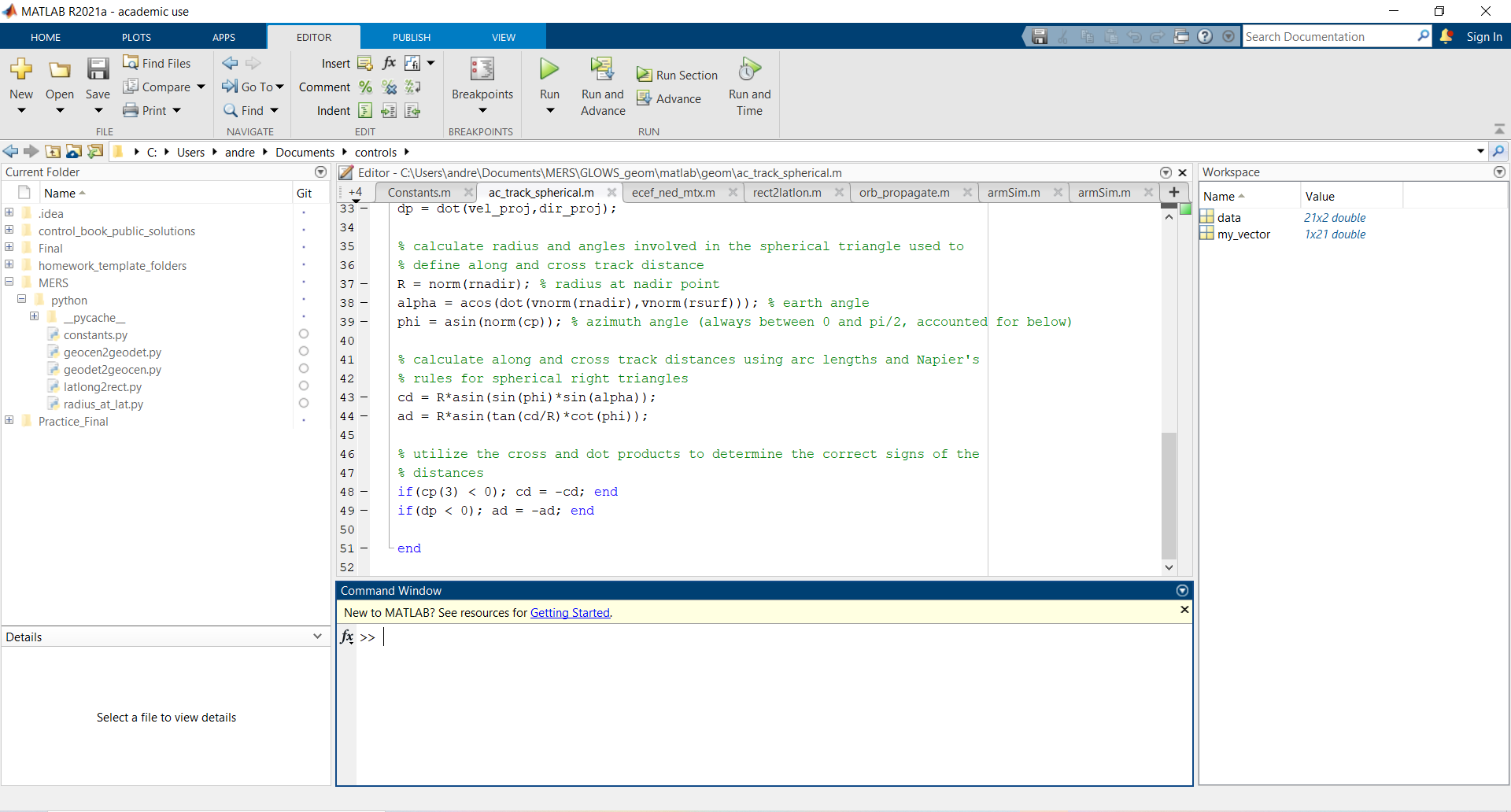
When first opening Matlab it can be overwhelming to a new user. The key sections of the matlab screen are the folder directory (left), the command window (bottom), the workspace (right), and the editor (middle top). The folder directory is used when accessing a directory of files, which is especially common with large Matlab programs which hold many Matlab scripts which will allow for easy navigation between files. The command window is where one can directly write in Matlab commands and run them. The Workspace is similar to a stack frame as it is an area where local variables are stored for easy access and reuse. The editor is used in creating and editing Matlab scripts.

Basics

Other more “standard” coding languages (such as C++ and C) require a file to be converted from source code to an executable file before it can be run. They are thus referred to as a compiled language. In contrast, Matlab is known as a scripting language or an interpreted language (similar to Python or Java) in that the code that is written can be immediately run through a Matlab suitable terminal and the lines of code will be executed as is (by means of an interpreter).

While for any project it is technically possible to write entire programs line by line and execute them in the command window it is generally good practice to write Matlab scripts (denoted by .m file endings) which contain many lines of Matlab code which can then be run sequentially.

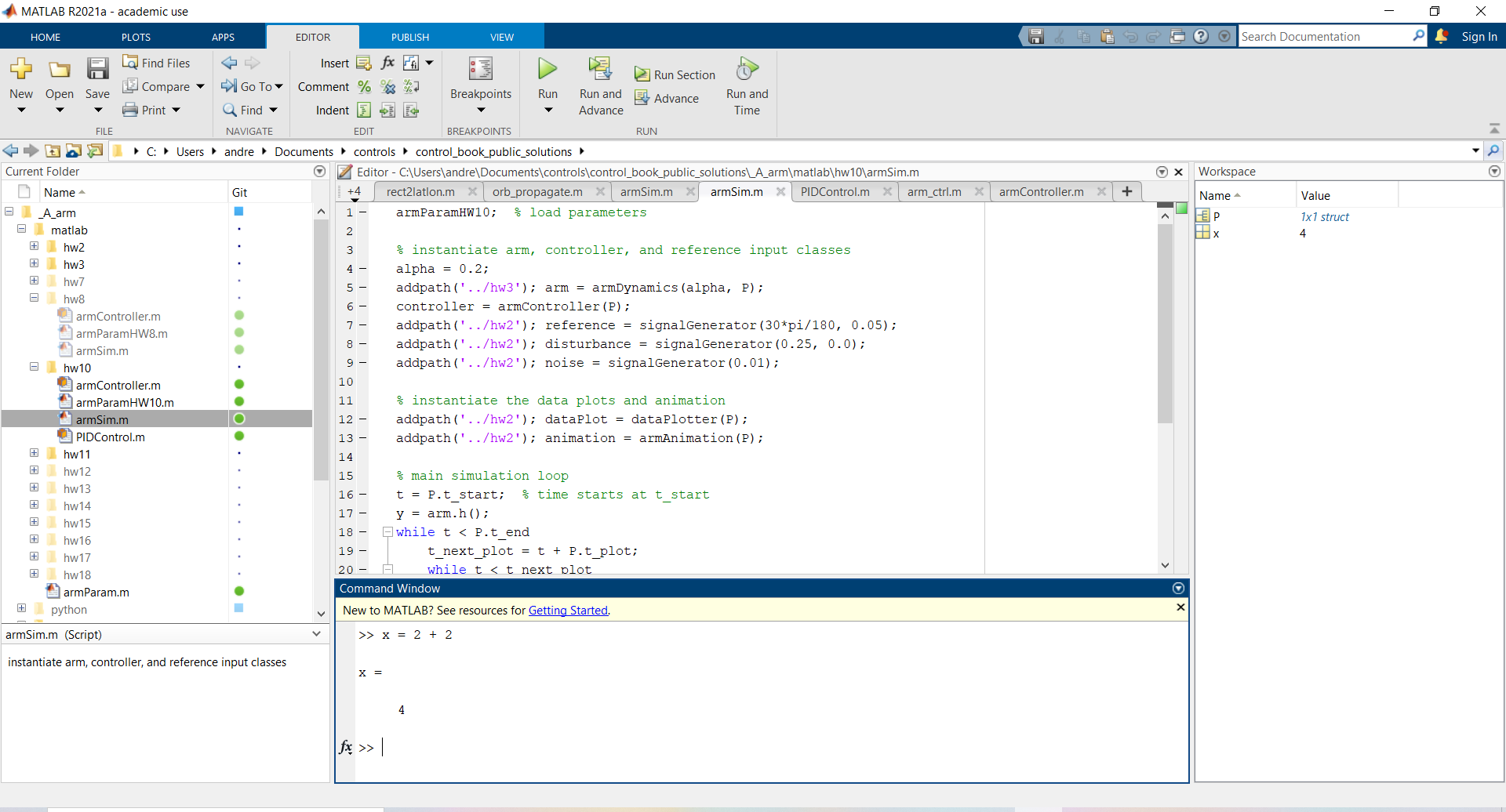
One key characteristic of Matlab is the use of the semicolon ;. The semicolon suppresses the output of a command. For example:

If the following command is run in the terminal window

  x = 2 + 2

the variable x is assigned the value (2 + 2) or 4, and the output is printed to the command window as shown below:

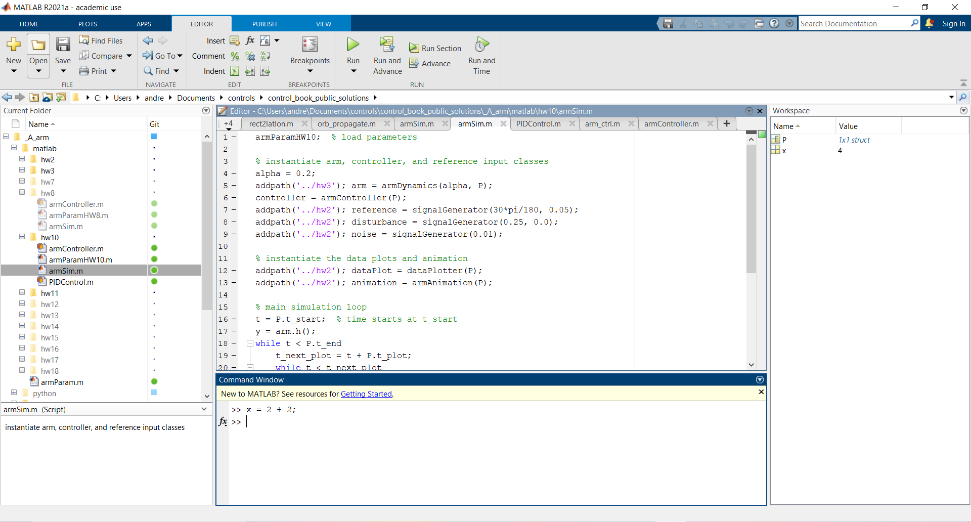
In contrast if a semicolon is placed at the end of the line:

  x = 2 + 2;

the variable is assigned the value (2 + 2) or 4 the same as above, but the output is suppressed and does not display in the command window.

Below are some other helpful commands to be used:

• help
• clc
• close
• clear
• edit

Below are some other helpful resources for beginners to Matlab:

• Introduction to Matlab
• MATLAB Quick Reference

Basic plotting

2-D plots

Matlab offers a number of plotting capabilities. The basic 2-D line plot requires the use of vectors, which can be created by using the form (starting point):(increment):(ending point). For example, the vector

  my_vector = 0:5:100;

creates a vector starting at zero, ending at 100, which is incremented up by 5.

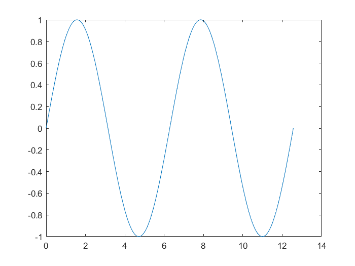
plot(x,y) creates a line-plot of the vectors x and y. Make sure vectors x and y are of equal length. For example, the vector

  x = 0:pi/50:4*pi;

creates a vector starting at 0 and incrementing up to 4 pi.
The vector

  y = sin(x);

creates a vector that has values that are the sine of the values in vector x.
We can then use the command

plot(x,y);

to graph vector y versus x:

Adding a title and axis labels can be achieved using the following commands:

  title('This is a Title');
  xlabel('My x-axis label');
  ylabel('My y-axis label');

To plot multiple functions on the same graph, create the vectors for each function and use plot(x,y1, x,y2):

  x = 0:pi/30:4*pi;
  y1 = 2*sin(x);
  y2 = cos(2*x);
  plot(x,y1, x,y2);

legend(‘sine’, ‘cosine’) adds a legend to the side with the first label in the parenthesis corresponding to the first function in the plot command.

Try it

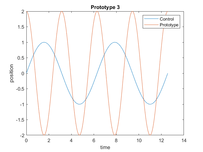
Using the commands shown, try to create a graph to look like the following picture.

3-D plots

plot3(X,Y,Z) plots a function in 3-D.

The commands

  x = 0:0.1:30;
  y = sin(x);
  z = cos(x);
  plot3(x,y,z);

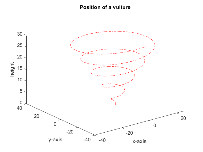
produces the following graph:

The style and color of the line can be changed by adding another argument in the plot function. For example,

plot3(x,y,z,'--');

produces a 3-D plot with a dashed line.

Try it

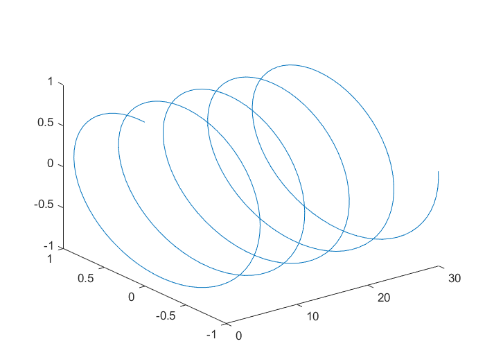
Try to recreate the following image. (Hint: use .* to multiply an element of one vector by an element of another vector)

Surfaces

surf(X,Y,Z) produces a 3-D surface with solid face colors. This function plots the values of matrix Z as a height of a grid on the x-y plane formed by using the meshgrid command. The surface’s color changes depending on its height.

The command colorbar displays a bar to reference the values of the different colors of the surface, and axis([limit]) can change the axis of the plot.

For example, the commands

[X,Y] = meshgrid(0:0.1:10,0:2:20);
Z = sin(X);
surf(X,Y,Z);
axis([0 10 -5 25 -2 2]);
colorbar;

creates the following surface:

Try it

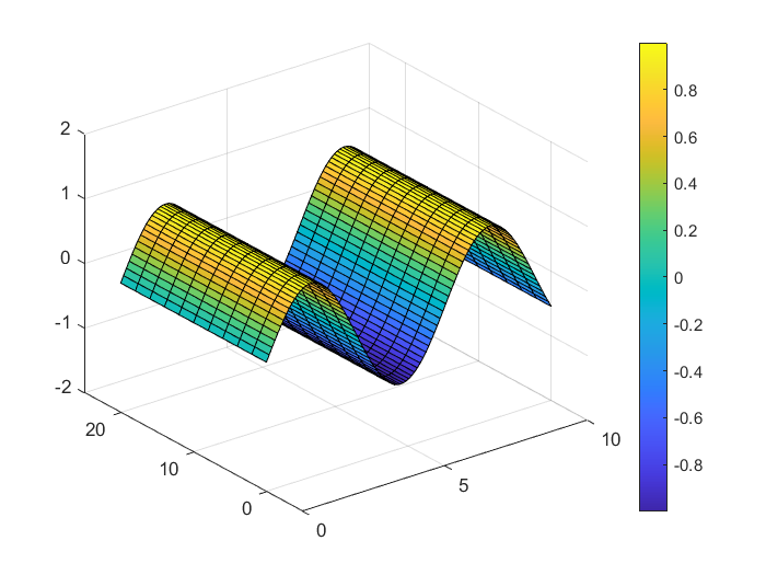
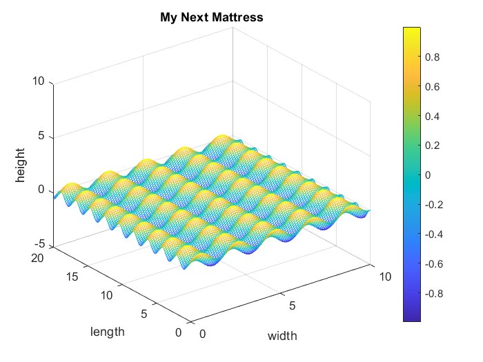
Using one of the other surface and mesh plots, as well as a certain combination of a sine and cosine function produces the following surface:

Learn more about plotting in Matlab:

• MathWorks plot Help Center
• BYU ECEn 240 Matlab Intro
• Tutorialspoint Matlab Plotting
• Create the MATLAB logo

Manipulating Matrices

A matrix is a rectangular array or table of numbers, arranged in rows and columns. Matrices can be very useful if you know how to use them in various calculations. Luckily MATLAB will do some of those calculations for you. We’ll start with the basics of creating matrices and accessing values within the matrix.

Creating a 3x4 matrix

  a = [ 1 2 3 4 ; 2 3 4 5 ; 3 4 5 6 ]

will output the following matrix:

  1 2 3 4 
  2 3 4 5 
  3 4 5 6 

To access a value within a matrix use the following. Note that all indexing in MATLAB starts at i=1.

  temp = matrixName(row,col)

You can also access a range of values within a matrix by using a colon. If you have just the colon, it will select the entire row/column. You can also specify the range using the expression

  startIndex:endIndex

This will start with the first index listed and includes the last index included. Below are examples of accessing values within a matrix. Think about what the code will print,try it in MATLAB, and see if you got the desired results

  a = [ 1 2 3 4 ; 2 3 4 5 ; 3 4 5 6 ]
  index1 = a(2,3)                        % 4
  index2 = a(3,1)                        % 3
  index3 = a(:,3)                        % 3 4 5 (will be printed vertically)
  index4 = a(2,:)                        % 2 3 4 5
  index5 = a(1:2,3)                      % 3 4 (will be printed vertically)
  index6 = a(:,1:2)                      % 1 2 ; 2 3 ; 3 4 (will be printed vertically)

You can also manipulate matrices by deleting rows/columns and creating submatrices. To delete a row/column you set it equal to an empty array

  a(2,:) = []                            % 1 2 3 4 ; 3 4 5 6 

To create a submatrix you set a new matrix equal to the range of the old matrix you want

  new_a1 = a(2:3,1:4)                    % 3 4 5 ; 4 5 6 

You can also create a new matrix by using lines from previous matrix. The following code will take matrix a and turn it into a 3x3 matrix while using row 2 for the first and last row

  new_a2 = a([2,1,2],1:3)                % 2 3 4 ; 1 2 3 ; 2 3 4 

Try it

Using the following matrix and the commands you just learned, find the following:

try_it = [ 2 1 4 3 ; 4 1 2 1 ; 1 3 4 2 ]

• What are the index of all occurrences of the value 2 ( SOLUTION: (1,1), (2,3), (3,4) )
• Sum of row 2 and 3 ( SOLUTION: [ 5 4 6 3 ] )
• Column 4 multiplied by the value in index (1,2) ( SOLUTION: [ 3 ; 1 ; 2 ] )
• Index (3,4) multiplied by the 2x2 matrix in the bottom right corner ( SOLUTION: [ 4 2 ; 8 4 ] )
• Create a 3x3 submatrix ( SOLUTION: [ 1 4 3 ; 1 2 1 ; 3 4 2 ] - answers may vary )
• Delete the first column and last row ( SOLUTION: [ 1 4 3 ; 1 2 1 ] )
• Turn the 3x4 matrix into a 4x4 matrix repeating the last row twice ( SOLUTION: [ 2 1 4 3 ; 4 1 2 1 ; 1 3 4 2 ; 1 3 4 2 ] )

Matrix Operations

Here are a few commonly used matrix operations. We will use the following matrices in the examples:

  a = [ 1 2 3 ; 4 5 6 ; 7 8 9 ]
  b = [ 5 1 2 ; 4 5 1 ; 2 6 3 ]
  c = [ 2 -3 1 ; -1 2 0 ; 2 2 1 ]

• Addition

  a + b              % 6 3 5 ; 8 10 7 ; 9 14 12 (will be printed vertically)
  

• Subtraction

  a - b              % -4 1 1 ; 0 0 5 ; 5 2 6 (will be printed vertically)
  

• Scalar operations

  a + 3              % 3 5 6 ; 7 8 9 ; 10 11 12 (will be printed vertically)
  a - 3              % -2 -1 0 ; 1 2 3 ; 4 5 6 (will be printed vertically)
  a * 3              % 3 6 9 ; 12 15 18 ; 21 24 27 (will be printed vertically)
  a / 3              % 0.3333 0.6667 1.0000 ; 1.3333 1.6667 2.0000 ; 2.3333 2.6667 3.0000 (will be printed vertically)
  

• Transpose

  a'                 % 1 4 7 ; 2 5 8 ; 3 6 9 (will be printed vertically)
  

• Concatenate

  [ a , b ]          % 1 2 3 5 1 2 ; 4 5 6 4 5 1 ; 7 8 9 2 6 3 (will be printed vertically)
  [ a ; b ]          % 1 2 3 ; 4 5 6 ; 7 8 9 ; 5 1 2 ; 4 5 1 ; 2 6 3 ] (will be printed vertically)
  

• Multiplication

  a * c              % 6 7 4 ; 15 10 10 ; 24 13 16 (will be printed vertically)
  

• Determinant

  det(c)             % -5
  

• Inverse

  inv(c)             % -0.4000 -1.0000 0.4000 ; -0.2000 0 0.2000 ; 1.2000 2.000 -0.2000 (will be printed vertically)
  

Learn more about matrices in Matlab:

• Tutorialspoint
• MathWorks Arrays vs Matrices