Table of Contents
In this two-part lab you will implement a Differential Power Analysis (DPA) side channel attack on DES encryption.
Preliminary
DPA
While SPA attacks are effective when the implementation leaks significant information through power consumption, many implementations employ countermeasures to prevent this. Differential Power Analysis (DPA) attacks are more powerful and can be used against a wider variety of implementations. DPA attacks extract information from more subtle correlations between the power consumption and the data being processed. These variations tend to be smaller and are sometimes overshadowed by measurement errors and other noise. In such cases, it is still often possible to break the system using statistical functions tailored to the target algorithm.
In an acquisition campaign, m power curves, $T$, (also casually called “traces”) are garnered. Each trace, $T_i$, corresponds to a given leakage of the device when processing a known input (plaintext or ciphertext). For the sake of simplicity, we focus on a part of the leakage, related to a very restricted set of gates in the netlist. We assume this leakage can be summarized into two typical behaviors: high dissipation to charge a net versus low dissipation to discharge it, and activity versus no-activity.
These two behaviors are related to an inner Boolean variable, called a decision (selection) function $D_i$. If the secret key is unknown, this variable is also unknown; however, it depends in practice on only a couple of bits from the key, which can be tested exhaustively. The decision function $D_i\in\lbrace 0,1\rbrace$ is an oracle for an attacker: if it is the correct decision function, it can allow for an exhibition of the two behaviors, otherwise it is simply irrelevant. The idea behind DPA is to exhibit an asymptotic difference between the behaviors.
The ad hoc criterion is defined as:
\[DPA = \frac{1}{m_0} \sum_{\substack{i \\ D_i = 0}} T_i - \frac{1}{m_1} \sum_{\substack{i \\ D_i = 1}} T_i \tag{1}\]Where $m_0$ and $m_1$ denote the number of traces for each decision.
DPA Attack on DES
Paul Kocher defined the selection function $D(C, b, K_s)$ as computing the value of bit $0 \leq b \leq 32$ of the DES intermediate $L$ at the beginning of the 16th round for ciphertext $C$, where the 6 key bits entering the S box corresponding to bit $b$ are represented by $0 \leq K_s \leq 2^6-1$. Note that if $K_s$ is incorrect, evaluating $D(C, b, K_s)$ will yield the correct value for bit $b$ with probability $P \approx \frac{1}{2}$ for each ciphertext.
The attack can be done on the 16th round using the ciphertexts ($C_{1..m}$) or on the 1st round using the plaintexts ($P_{1..m}$). In this lab it’s a bit easier to do the attack on the 1st round using the plaintexts, so we will use the decision function notation $D(P, b, K_s)$ below.
To implement the DPA attack an attacker first observes $m$ encryption operations and captures power traces $T_1,\dots,T_m$. Each trace $T_i$ contains $k$ samples $T_i[1..k]$.
DPA analysis determines whether a key-block guess $K_s$ is correct by computing a $k$-sample differential trace $\Delta D[1..k]$. Let $D_i \equiv D(P_i,b,K_s)$ be the selection value for the $i$-th plaintext $P_i$ and bit index $b$. Let $m_0$ and $m_1$ be the counts of traces with $D_i=0$ and $D_i=1$.
\[\Delta D[j] = \frac{1}{m_1}\sum_{\substack{i\\D_i=1}} T_i[j] - \frac{1}{m_0}\sum_{\substack{i\\D_i=0}} T_i[j].\]Thus $\Delta D[j]$ is the difference between the mean sample at time $j$ for traces with $D=1$ and the mean for traces with $D=0$.
If $K_s$ is incorrect then $D_i$ equals the true target bit about half the time, so $D$ is effectively uncorrelated with the device’s internal bit.
For a random split the difference of the subset means tends to zero in probability as $m\to\infty$.
If $K_s$ is correct then $D_i$ equals the actual target bit (with probability 1 in the ideal model) and $\Delta D[j]$ converges to the contribution of that bit to the power signal as $m\to\infty$. Uncorrelated noise and other data contributions average out. The plot of $\Delta D$ therefore shows spikes at sample indices $j$ where the target bit causes observable power transitions.
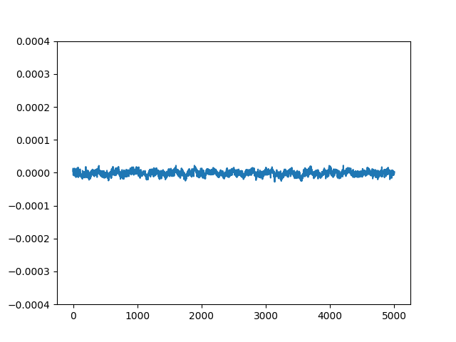
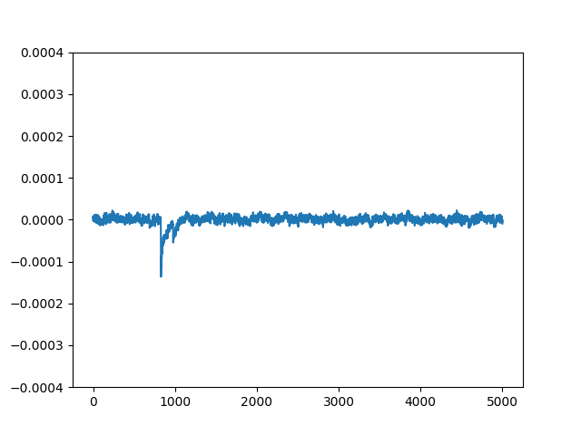
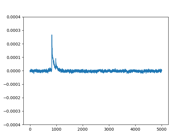
The images below show three example $\Delta D[j]$ traces. The first trace is for an incorrect key guess that produces no significant spikes. The second trace is for another incorrect key guess that produces some small spikes due to the guessed key producing correct $D$ values for some of the traces by chance. The third trace is for the correct key guess that produces a significant spike at a particular sample index. When you guess all possible key values and compute $\Delta D[j]$ for each guess, the correct key will be the one that produces a trace with the largest absolute spike (positive or negative) at some sample index.
Power Traces
In this lab, you do not need to take any physical measurements. To do a DPA, from hundreds to tens of thousands of measurements are required. We don’t have time to do that many measurements in this experiment. Therefore, you will process the data provided to you. There are in total about 80000 traces provided. Download this file. Place the traces.npy file in the lab_dpa_i/ directory.
They are the power consumption traces that include an entire DES operation of 16 rounds. Each trace contains both the plaintext and ciphertext (although we only need one of these to perform the attack – in this lab we will only use the plaintext to perform the attack).
The traces can be loaded in Python using the provided read_traces.py file.
import joblib

# plain:    a list of 81569 plaintexts.  Each plaintext is a 16-character hex string
# cipher:   a list of 81569 ciphertexts. Each ciphertext is a 16-character hex string
# voltages: numpy ndarray. The first dimension is the number of traces (81569),
#           the second dimension is the number of samples in each trace (5003)
plain, cipher, voltages = joblib.load("traces.npy")
The provided traces are very similar to what is shown below. You can plot a trace like so:
import matplotlib.pyplot as plt

plt.plot(voltages[0])
plt.title("Voltage Trace 0")
plt.xlabel("Sample")
plt.ylabel("Voltage")
plt.show()
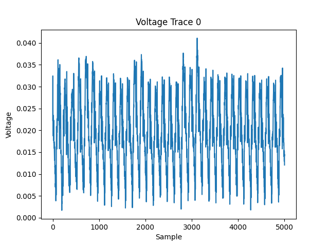
As these 80000 traces are obtained when the DES are encrypting different plaintext (with the same key), the waveforms are different from each other. However, you can hardly tell the difference by looking with your eyes. If you do subtraction between two traces, you can see they can almost cancel out each other.
DPA With Python
The first step of DPA is to divide these traces into two groups using your selection function. Then, for each group, you can calculate a new trace, that is the average of all traces in the group. This can be done easily using in numpy; like so:
group1_avg = np.average(group1, axis=0)
These two average traces may still look very similar to the trace above. However, with an average trace computed for each group, you can calculate a new array, which is the difference between the two groups. Again, this is very easy in Python:
diff_trace = group1_avg - group2_avg
When you calculate the difference between these two average traces and plot out the difference, an exciting thing happen. If you divided the traces using the right way in the first step, you can see that these two average traces cannot cancel out each other anymore. There will be a peak, which may be positive or negative. You can easily plot a trace with matplotlib:
plt.plot(diff_trace)
plt.show()
The key point is how you divide these traces into two groups. If you divide them randomly and calculate the difference of the average trace for the two groups, they cancel each other out. If you divide them the wrong way, there may be no difference from a random partitioning. You should design a good selection function which, if the key guess is right, can divide the traces in a correct and efficient way, so that the two average traces cannot cancel each other.
DPA Details for DES
How do we design the selection function? We know that the DES does the same operation for 16 rounds and the weakness of DES is always in the first round or the last round. (Why?) In this experiment, we will try to recover the sub-key for the first round, through guessing and checking the difference trace. Once we know a sub-key for one round, we can calculate out the original key. In this lab, you will figure out the round 1 key, and in next week’s lab, you will use this to figure out the full key.
We also know that semiconductors use current while switching. We can concentrate on one bit of one register (register R shown in the left figure below recommended). Register R begins as the right-hand side of the input plaintext, after the input permutation, referred to as R0 in the figure. The first round concludes with register R being updated to a new value (R1). We will use the hypothesis that if a bit in R flips from R0 to R1, then there will be a different power signature than if it does not change. If a given bit in R flips during the first round, we put the trace into one group. If it doesn’t flip during the first round, we put it into the other group. Therefore, after we put all the traces into these two groups correctly, the traces in one group all tend to consume more power (at an unknown but certain time), and there will be a peak (at that certain time) in the difference trace.
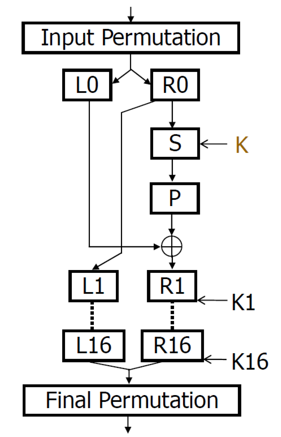
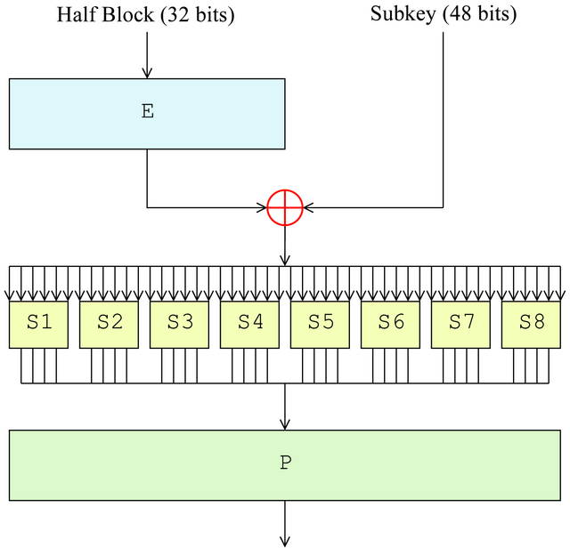
Now we can design the selection function. The function will take 3 inputs: what the plaintext (M) is, which bit (1 ≤ 𝑏 ≤ 32) of register R you choose to inspect, and your guess for the round 1 subkey, K. While the round subkey is 48-bits (which is too large to try all guesses), if you inspect the DES algorithm (the right figure above shows some of the details of the S box from the left figure), you will see that each bit of R1 comes from one of the eight substitution boxes (s-boxes), and each s-box is influenced by a unique 6-bit range of the 48-bit round key. This means that you can guess the round subkey 6 bits at a time, making the attack quite feasible. For each 6-bit s-box key, you will need to try all combinations (0 ≤ 𝐾sbox 𝑖 ≤ 63), and perform a partitioning of the traces for each key guess. The one with the biggest peak will be the right guess. You will then repeat this for each sbox (8 times).
The bit you inspect ($b$) can be chosen by you. Each s-box influences 4 bits of the 32-bit R register, so make sure you choose one of these 4 bits that are relevant to the s-box you are targeting. Note that after the 8 s-boxes finish their substitution, there will be a permutation (the P box in the figures above). That means the 4-bit output of the first sbox (which operates on the most significant 4 bits of R0), will NOT go to the most significant 4 bits of R1. You will need to careful when selecting $b$ to be sure the bit you watch in R is influenced by the sbox you are targeting.
Instructions
- REPORT: The first round and last round of encryption algorithms are often targeted by hackers. Why are these rounds often the weakness?
- REPORT: Which bits in R1 will the first sbox’s output go to? Refer to the DES code to answer this question (Here “first” means this sbox takes the 6 most significant bits from the XOR result of the sub key). Make sure to answer it correctly. Your DPA attack won’t work without choosing an appropriate bit in the R register to watch, when trying to guess the 6-bit portion of the round key.
- Create a python script that works to determine the 6-bit key for the first sbox
- Choose a bit from the previous question as $b$.
- Create a selection function in Python. The output of the function is either 0 or 1. If bit $b$ stays the same during the first round (from R0 to R1), the output is 0. If bit $b$ flips, the output is 1.
- Try all 64 values for the 6-bit sbox key.
- Identify the 6-bit sbox key that produces the largest peak.
- Repeat this process for each of the remaining 7 sboxes.
- For each sbox, you will need to choose a new $b$ bit-index to use for your selection function. Make sure to select one that is appropriate for the sbox you are targeting.
- REPORT: For each sbox, add the trace difference graph to your report showing the key ($K$) value that produces the highest peak, as well as the trace difference graph when $K=63$. This is a total of 16 graphs.
- REPORT: In your report, provide the round1 key that you have obtained. Provide this as a list of 8 6-bit keys, in decimal, from most significant to least significant. Example: (23, 62, 7, 36, 2, 50, 41, 14)
What to Submit
Tag your submission as lab_dpa_i and make sure to commit:
- Your lab report (
lab_dpa_i/report.pdf). - Your Python files for the DPA attack (place them in
lab_dpa_i/).
Helpful Tips
Python Packages
You will need several Python packages to complete the lab. I recommend you create a Python virtual environment to install these packages. A Makefile has been provided in the lab_dpa_i/ directory that will create a virtual environment and install the necessary packages. Run:
make env
to create the virtual environment, and
source .venv/bin/activate
to activate it in your terminal.
DES Selection
This lab requires you to determine R0 and R1 values internal to the DES algorithm. Rather than having you implement this portion of the DES algorithm, I suggest you use a pre-existing implementation, and then modify it as needed. I have provided des.py in the lab_dpa_i/ directory that you can use. This code is from https://medium.com/@ziaullahrajpoot/data-encryption-standard-des-dc8610aafdb3.
I suggest copying the encrypt function to a new function that simply returns the R0 and R1 values (keep the original encrypt function in case you need it later). You can return immediately after the R1 value is computed as you don’t actually need the remainder of the DES algorithm. Add an additional parameter to the function that allows you to override the round one key with a provided binary string. With this in place, it will be simple to create a selection function that sorts the power traces based on whether your bit of choice changes from R0 to R1.
DES Implementation
You may want to look back to your lab_trojan_i/des.v and lab_trojan_i/crp.v files for reference on how the DES algorithm works.