Implement the FIR and IIR Filters

Overview
Resources
1. Source Code
Implementation Details
Test Code
Pass Off and Code Submission
Notes to TAs

Overview

Now that you have designed your FIR and IIR filters using MATLAB, you will implement these filters using C-code that executes on the the laser tag unit. In support, you will also implement a delay line component that allows retrieval of past filter sample values. You will verify the correct operation of your filters using test code provided in the ECEN 390 project directory.

Summary: What You Are Building

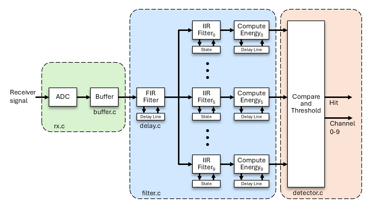
For Task 1, you are implementing just the signal processing component of the receive path. The diagram below shows you the entire receive path. You are implementing the part contained in the blue box, which consists of the following sub components:

Delay Line: a memory buffer for filter samples. Samples are saved in the order received and are retrievable by index relative to the most recently saved.
State: storage for saving intermediate values for each IIR filter.
FIR Filter: the decimating, anti-aliasing FIR filter.
IIR Filter 0-9: the IIR bandpass filters.
Compute Energy 0-9: compute the amount of energy in the signal output from the corresponding IIR filter.

The IIR-Filter and associated Compute-Energy components are now numbered 0 - 9 in this task. This is because ‘C’ arrays are zero indexed and starting at 0 makes coding easier. In MATLAB for Milestone 2, the frequencies and IIR filters were numbered 1 - 10.

General Requirements

Convert your filter coefficients developed in MATLAB to ‘C’ code.
You must implement all of the functions that are listed in delay.h and filter.h.
You must follow the coding standard.
Your FIR filter must have a reasonably flat frequency response up through 5 kHz and then should quickly roll off.
Your IIR filters must have a very narrow frequency response. For example, for frequency 4, your energy output should be high for IIR filter 4, but should be very low for all of the other IIR filters. A difference of 10X is preferred for good performance in the laser-tag game.
You must demonstrate the behavior of your filters and energy-computation functions to the TAs using the provided source code.

General Notes

Assume a sample rate of 80 kHz for the input to the FIR filter.
The decimation rate for the FIR filter is 8.

Filter Coefficients

To get started, you will need the filter coefficients from Milestone 2.

One set of coefficients for the FIR filter code.
Ten sets of coefficients for the IIR filter code. Each IIR coefficient set consists of a few second-order sections (which in turn consist of b and a coefficients).

Resources

Source Code

Note that the following files are provided in your ecen390 project directory. The test code is used to check the correctness of your code.

ltag/main/delay.h
ltag/main/filter.h
ltag/main/main_m3t1.c
ltag/main/test/test_delay.h
ltag/main/test/test_delay.c
ltag/main/test/test_filter.h
ltag/main/test/test_filter.c
ltag/components/histogram/histogram.h
ltag/components/histogram/histogram.c

These coefficient files can be created by running a provided MATLAB conversion script.

ltag/main/coef.h
ltag/main/coef.c

You are expected to create and implement the following files. See the provided header files (.h) for a description of each function.

ltag/main/delay.c
ltag/main/filter.c

When implementing each function, pay attention to the function descriptions in the header files. In fact, save lost points from the coding checker by copying the comments and function prototypes from the header files to your .c files to start your code. Also, you are likely to lose points from the coding checker if you modify the header files! So, don’t modify the provided header files.

Implementation Details

Convert Filter Coefficients to C Code

A MATLAB script is provided to assist you in converting your filter coefficients developed in Milestone 2 to ‘C’ code.

Input:

FIR filter coefficients saved as a .mat file.
- FIR_b is a 1 x N vector of single-precision floating-point values.
IIR filter coefficients saved as a .mat file.
- IIR_sos is an F element cell array of S x 6 single-precision matrices.
- F is the number of IIR filters, one for each player frequency.
- S is the number of second-order sections in the filter.
- Each section contains 6 coefficients {b0, b1, b2, 1, a1, a2}.

Output:

coef.h - header file with array declarations and #defines for sizes.
coef.c - ‘C’ file with initialized arrays named fir_b and iir_sos.
- Each second-order section contains 5 coefficients {b0, b1, b2, a1, a2}.
  - The first a coefficient equal to 1 is dropped.

The process is simple if the above input assumptions apply to your saved MATLAB coefficients. If not, you can modify your MATLAB code or modify the conversion script so that they match.

Instructions:

Download the MATLAB script coef.m into the same directory you used to design your filters.
Run the script to format your coefficients into ‘C’ arrays.
Copy or move the generated coef.h and coef.c files to your ecen390/ltag/main directory.
When implementing filter.c, include coef.h at the top of your file so you can access the filter coefficients.

Delay Code

The delay component implements a delay line. It acts like an array of elements of size N that gets shifted down (to the next higher index) each time a new element is saved at index zero. The last element in the array falls off the end when shifted. An element retrieved from index zero is the most recent element saved. Each higher index goes back in time by one time step. The actual implementation uses a circular buffer.

In delay_init(), use malloc() to allocate memory for the delay line and then check to see if the allocation failed. Also, make sure that the allocated memory is initialized to zero. malloc() does not initialize the returned memory to zero.

/* in delay_init() */
d->data = malloc(size * sizeof(delay_data_t));
if (d->data == NULL) abort();

The pos member of the delay_t struct, should be initialized to zero. When a new value is saved to the delay line, decrement the position pos and then store the value. If a decrement would cause the position to go negative, wrap around and set the position to the delay line size (in elements) minus one.

Do not implement the delay component by shifting values. It will be too slow!

Filter Initialization

As each signal sample is processed through the filter stages, memory is needed by each filter to keep a running history of sample values to multiply against the filter coefficients. Additionally, for an IIR filter, memory or “state” is needed to hold feedback from the output. To compute the energy in the output signal of each IIR filter, a history, or sliding window, of sample values is also needed. Use instances of the delay component to maintain the history of values needed for the FIR filter and energy computation. There should be one instance for the FIR filter and an array of instances for the energy computations. For the IIR filter, use a 3D array to hold the state. The size of the first dimension is the number of filters, the second is the number of second-order sections, and the third is the number of state variables.

#define SOS_STATE 4 // Number of state variables per second-order section
static filter_data_t iir_state[IIR_FILTERS][IIR_SOS_SECTS][SOS_STATE];

Use filter_init() to initialize each instance of the delay component by calling delay_init(). Also, initialize an array of current energy values to hold the output of the energy computation, one array element for each IIR filter.

The filter_reset() function only sets the delay and state memories to zero without allocating memory. It should call delay_reset() to reset the delay instances. The 3D array of IIR state can be set to zero with one call to the memset() function. Also, set the current energy values to zero.

Filter Code

Background

In this task you will implement the FIR and IIR filters that you designed with MATLAB in ‘C’ code. Let’s start with the FIR filter. Remember that the FIR filter is implemented as a weighted sum of some past number of inputs. Here’s an example from Wikipedia:

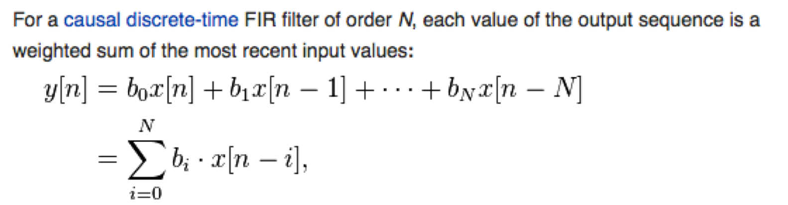
It can be confusing to transition from the finite array-based approach used in MATLAB to the “infinite” approach that is required in the implementation of a signal-processing system. The inputs and outputs of a real-time signal-processing system are essentially infinite. As such, the array-based notation in the equation above fails us because the output is an indexed array y[n]. For example, at time=0, you start out computing y[0]. After playing the game for several minutes, n would be in the billions. And, it only goes up from there. Simply put, you want to eliminate the [n] part so that the output is simply y.

Note that in the English-based description from Wikipedia (see above), indexes were not discussed. Remember that the FIR filter is implemented as a “weighted-sum of some past number of inputs”. All those indexes, the i, the k, etc., are just a way to keep the coefficients properly aligned with the data. The goal is to keep the recent history of input values aligned with the coefficients.

The idea is pretty simple and is based upon these ideas:

Create a delay line structure that will keep an ordered history of past values. The size of the data structure must match the order of the filter, e.g., a 50-tap FIR filter needs a history of 50 values.
At start-up time, initialize the delay line with zeros.
As each new value arrives, throw away the oldest value.
Read the stored, past values from the delay line and multiply them with the correct coefficients.

FIR Filter

You can implement a FIR filter using the delay line as described above. Consider an example where the FIR filter uses N of the most recent input values to compute its output. N is equal to the number of b coefficients.

Assume:

fir_b is an array of b coefficients for the FIR filter
FIR_B_COEFS is the number of b coefficients in fir_b
fDelay is a delay line of size FIR_B_COEFS holding the most recent samples
in is the most recent sample from an ADC
output is the filter output for the current time step

#include "coef.h"
#include "delay.h"
#include "filter.h"

  ...
  delay_save(&fDelay, in);
  filter_data_t output = (filter_data_t)0.0;
  for (delay_size_t i = 0; i < FIR_B_COEFS; i++) {
    output += delay_read(&fDelay, i) * fir_b[i];
  }
  ...

The purpose of the delay line is to store past values in the order that they were received and make all of the contained values accessible during the filter computation.

What About Decimation?

Decimation is really easy. In our laser-tag system, we will be decimating by 8. All we do is invoke our FIR filter each time we receive 8 new samples. As you save incoming samples to the FIR-filter delay line, only invoke the FIR filter each time you have received 8 new inputs. Use the run argument to filter_firFilter() to control when it should invoke the filter. This function should be called for each new input sample so it can be saved in the delay line, but run should only be true for every 8th sample.

IIR Filters

The difference equation (Direct Form I) for a second-order section of an IIR filter is shown below.

y[n] = b0 * x[n] + b1 * x[n-1] + b2 * x[n-2] - a1 * y[n-1] - a2 * y[n-2]

IIR filters of higher order are implemented as a cascade of second-order sections.

The implementation of the IIR filter is similar to the FIR filter. However, the IIR filter relies on two signal histories: x and y, as shown in the equation above. As you can see from the equation, you would need two delay lines to keep the necessary signal histories. The only other difference is that the computed value y is also saved to the delay line that keeps a history of y values. This is essentially what puts the “IIR” in the filter, e.g, feedback.

For the IIR filters, we will not be using the delay component for the signal histories, but rather a 3D array as described in Filter Initialization. In this case, we will be shifting the values in the “state” memory as a part of the filter code.

Below is a sketch of code that shows you how to “cascade” each of the second-order sections together apply the IIR filter to one incoming sample.

filter_data_t filter_iirFilter(uint16_t chan, filter_data_t in)
{
    ...
    // Cascade the results of each second-order section
    for (int8_t section = 0; section < IIR_SOS_SECTS; section++) {
        ...
        const float *c = iir_sos[chan][section]; // 5 coefficients
        float *w = iir_state[chan][section]; // State variables
        ...
    }
    ...
}

The temporary pointers c and w point to the coefficients and state variables need for the section being processed.

c: coefficients {b0, b1, b2, a1, a2}, c[0] is b0
w: state {x[n-1], x[n-2], y[n-1], y[n-2]}, w[0] is x[n-1]

Again, elements of the w array (e.g. w[0], w[1], …) will need to be shifted as a part of your IIR filter code for each sample processed.

Other forms of the IIR filter can be implemented with the advantage of only needing two state variables per section:

Computing Energy

Implement all of the energy-related functions (they all have the word “Energy” in their names). You will need to make sure to implement filter_computeEnergy() with an incremental approach so that it does not take too much execution time. Carefully think about how you might be able to reuse computations performed in a previous invocation of filter_computeEnergy() to reduce overall computation time.

To compute energy, you must keep a running history of 200 ms of output data from each of the IIR bandpass filters. Use a delay line instance for each IIR filter to hold this data. The size should be sufficient to hold 200 ms of samples. The energy for a signal contained in a delay line is the sum of the squares of all values.

Incrementally compute the energy from sample values contained in the energy delay lines. Since the delay lines eDelay[chan] and current energy values currentEnergy[chan] are initialized to zero, the incremental approach described below works from the start. Implementation sketch:

Read the oldest value from the delay line eDelay[chan] and call this old.
Save the newest value in, passed as an argument, to the delay line.
Compute a new energy as: currentEnergy[chan] - (old * old) + (in * in).
Save this energy as the currentEnergy[chan] and also return it.

Note that this function will need a global array currentEnergy[chan] to keep track of the current energy for each of the energy buffers.

Implement the filter_getEnergyArray() function which retrieves a copy of the current energy values. This function copies the already computed values into a previously-declared array so that they can be accessed from outside the filter pipeline by the detector. Remember that when you pass an array into a ‘C’ function, changes to the array within that function are reflected in the returned array.

Filter Pipeline

All the parts of the filter pipeline are brought together in the filter_addSample() function. This function adds a new sample to the filter pipeline and then runs each of the stages as necessary: decimating FIR filter, IIR filters, power computation. The filters are run when the sample count is a multiple of the decimation factor. The result of each power computation is saved internally and is retrievable with one of the getEnergy functions. filter_addSample() returns true if the filters were run.

Assume that this code is called whenever there is a new scaled ADC value available.

bool filter_addSample(filter_data_t in)
{
    static uint32_t sample_cnt = 0;
    bool run = ++sample_cnt == FILTER_FIR_DECIMATION_FACTOR;

    // Call the FIR filter function with the latest input sample
       // Set the run argument to true if the decimation factor was reached.
    // If run is true
       // Reset the sample count to zero
       // Run all the IIR filters and compute energy
    // End if
    // Return true if the filters were run
}

Test Code

To pass off this task, you must run your code with the provided test code. The test code calls functions in delay.c and in filter.c It also plots the frequency response for the FIR and IIR filters on the LCD display. In filter.h, you will see a section of code labeled “Verification-Assisting Functions”. These support functions provide a way for the test code to access the filter coefficients used in your filter.c code. These must be implemented.

Before building the test code, first set the MILESTONE variable in ltag/main/CMakeLists.txt to “m3t1”.

set(MILESTONE "m3t1")

Then, to build and run the tests, type the following:

idf.py build
idf.py flash monitor

The test results printed to a terminal window on the host computer will look like this if everything passes:

******** test_delay() ********
initialization test
save and read test
read out-of-bound test
reset test
******** test_delay() Done ********

******** test_filter() ********
filter_firFilter() alignment test
filter_firFilter() arithmetic test
filter_computeEnergy() test
filter_addSample() test
filter_addSample() average time:17 us
******** test_filter() Done ********

The “alignment test” checks that coefficient values are multiplied with corresponding delay line values using correct indices.

Along with the test results printed to a terminal window, the frequency response of the filters will be plotted on the LCD display.

Pass Off and Code Submission

You will show the TAs how your code behaves when running the provided test code. The test results will be displayed in a terminal window on the host computer. You will also show the TAs the information displayed on the laser-tag unit LCD.
You will submit your source code by doing the following:
1. From the top-level directory (e.g., ecen390), run ./check_and_zip.py m3t1.
2. The resulting .zip file will be in the top-level directory. Submit that to Learning Suite.
3. Submit only one .zip file per group. Both group members will receive credit.

Notes to TAs

Please pay attention to the following:

Check to make sure that both of the delay and filter tests pass.
Check to make sure that the plots on the LCD display look correct, e.g., the FIR-filter is flat across the frequency range and that the bandpass filters have a narrow response.