Design 10 Bandpass Filters
Table of contents
Overview
One of the essential parts of the laser tag signal processing system is the second stage, which consists of a bank of bandpass filters. In this task, you are going to design a bank of 10 bandpass filters and test them with simulated signals at the different player frequencies.
General Requirements
- Review IIR filter design
- Design 10 IIR bandpass filters centered at the player frequencies
- Analyze the performance of the 10 IIR bandpass filters and make sure that they meet the specifications
General Notes
For this stage of the signal processing system, assume your signal is already downsampled to 10 ksamples/s. Remember that the previous stage processed the signal at a higher sample rate before downsampling. Please pay particular attention to the specifications for the bandpass filters. Meeting these specifications is necessary for a functional laser tag unit and for uniformity between them when you actually use your laser tag unit for game play.
Specifications
The 10 bandpass filters should be IIR filters with the following specifications.
- Filter type: Butterworth bandpass filters centered at the player frequencies
- Player frequencies: 1250, 1481, 1739, 2000, 2353, 2667, 3077, 3333, 3636, 4000 (all in Hz)
- Filter order: 6 (or more in steps of 2)
- Filter form: Use second-order sections (SOS) for stability in single precision
- Bandwidth: 50 Hz or less between low and high cutoff frequency.
- Equal filter bandwidths for all 10 filters
- Attenuation:
- 3 dB (half-power) or more at +- 25 Hz around center frequency
- 40 dB or more for adjacent player frequency (at the center)
- Sampling frequency: 10 kHz
- Pulse length: 200 ms
- NOTE: A pulse length of 200 ms sampled at a frequency of 10 ksamples/s will yield a signal with 2000 total samples
Resources
Motivation
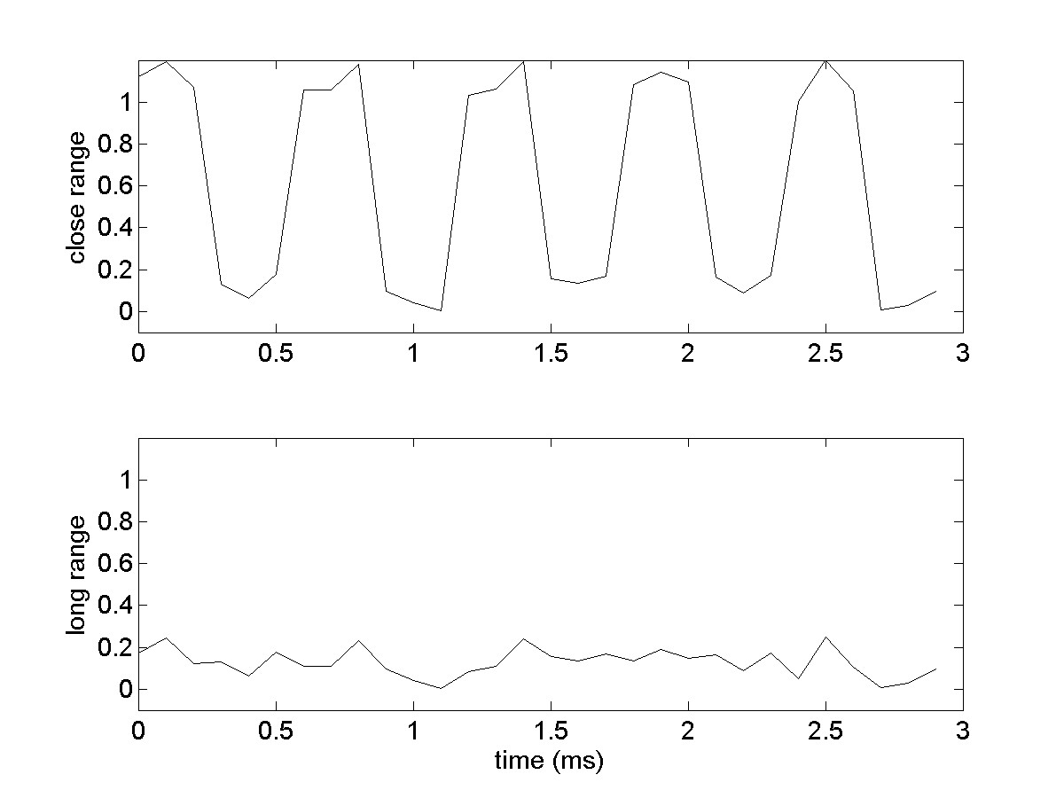
As you know, the laser tag system supports 10 players each with an assigned frequency in the range of 1.2 - 4.0 kHz. If the receiver is being illuminated or ‘hit’ by a laser tag beam then the sampled signal will consist of both a square wave at a particular frequency and noise. The system needs to analyze the received signal to determine whether the sampled signal contains a ‘hit’ by a laser tag unit. As the shooting unit gets farther away from the receiver, the amplitude of the square wave signal from the shooting unit gets smaller. Since the noise amplitude stays the same, this corresponds to a lower SNR, and it gets harder to distinguish the signal from the noise. This figure shows a square wave added to a random noise signal:

It will be easy for you to see the square wave in the close range signal, when the SNR is high. However, for longer-range signals, it will just look like noise even though there is a square wave embedded in the signal. The beauty of your signal processing system will be in its ability to detect a hit in the noisy received signal even at relatively large ranges.
The ‘hit’ signal has a frequency spectrum concentrated at the modulating frequency, while the noise is spread out over a wider frequency band. A simple method to extract the signal from the noise would be to compute a Fourier transform of the received signal, and then see if there is a spike in frequency at one of the player frequencies.
Unfortunately, computing a Fourier transform of the incoming signal requires too much computation time to enable it to be performed in real-time by our laser tag system. Therefore, we are effectively going to make a ‘coarse’ Fourier transform using our bank of 10 bandpass filters, and see if there is a spike in the signal energy coming out of any of the filters. This is computationally much more efficient, and can be implemented in real time (provided we keep the order of our filter low enough).
Filter Design
We are going to be using an Infinite Impulse Response (IIR) digital filter. The properties of an IIR filter are described on Wikipedia. An IIR digital filter is characterized by two sets of coefficients called ‘a’ and ‘b’. You may also want to review the sections on IIR filters in the ECEN 380 Discrete-Time Filters Lab.
There are lots of different filter designs that have already been developed. A few of the common types of filters are Butterworth, Chebyshev, and Elliptic. MATLAB has functions that produce the coefficients (a and b) for these filters. Let’s use the Butterworth filter for this example. A description of the Butterworth filter is available on Wikipedia. At the bottom of the Wikipedia page there is a comparison to the other common types of digital filters.
The first argument to the The MATLAB butter function represents one-half the filter order for bandpass designs. The next argument takes frequencies in units of half-cycles/sample. You can think of this as a normalized frequency in the range of 0 to 1, where one corresponds to half your sampling frequency. It simply tells you how many half-cycles your signal goes through per sample. The easiest way to get these normalized frequencies in half-cycles/sample is to divide your frequency in Hz by half the sample rate. I suggest keeping all of your frequencies in your MATLAB code as human readable Hz, and then simply divide your frequencies in Hz by half your sample rate when you pass them to the butter function.
Filter Creation
Since the laser tag system computes with single precision arithmetic, our IIR filter designs will need better numerical stability by using cascaded second-order sections (SOS). Another term for a second-order section is a biquad filter. Unfortunately, the butter function cannot directly output coefficients in SOS form. An extra step is needed. First, capture the filter coefficients in zero-pole-gain form. Then, convert them to SOS form using the MATLAB zp2sos function. Embed the gain in the first section. In addition, convert from double precision to single precision so that your analysis and simulation is more representative of the processing that will happen in the laser tag embedded system. You want to catch any numerical instabilities now in MATLAB and not when you are trying to program your laser tag system in ‘C’. A MATLAB cell array works well for storing the SOS matrix of coefficients for each of the 10 IIR filters. A sketch of the filter creation is shown below:
IIR_sos = cell(1, length(f_players)); % create cell array
% loop over each player frequency
    [zbp,pbp,kbp] = butter(...); % Butterworth filter
    IIR_sos{i} = single(zp2sos(zbp,pbp,kbp)); % convert to SOS
% end loop
The filter design parameters (what you can change) are:
- the filter type (i.e., Butterworth, Chebyshev, etc.),
- the filter order, and
- the cutoff frequencies.
To make it easier for the TAs to help, we are going to limit the number of design parameters. We want all to use the Butterworth filter design. Furthermore, we are going to limit the filter order to 6 so that your filters can operate in real time on the laser tag system. Note that this corresponds to 3 second-order sections (SOS) cascaded together. If the filter order is too high, it may not run fast enough on the laser tag system.
The only design parameter left to vary is the cutoff frequencies (based on the bandwidth) of the filters. Each Butterworth bandpass filter has two frequency corners. It should pass signals with frequency components between these two corners and attenuate other components. Next, create the bandpass Butterworth filter, and generate the second-order sections for the filter.
If we were performing true coarse frequency domain analysis, the filter would need to cover the entire band between the different player frequencies. However, in this system, we have a discrete set of allowable frequencies. The filter just needs to pass one of these allowable frequencies to see if the receiver is ‘hit’. Therefore, the bandwidth of the filter just needs to cover the specific allowable frequency that it is assigned. This means that for narrower bandwidths, more noise will be rejected and better system performance can be expected. However, this assumes that the frequency of the transmitter does not change at all. Therefore, we need to create some bandwidth to allow wobble in the player frequency. How much bandwidth is actually needed? After your laser tag units are built, experiments can determine the best bandwidth for your system. In this example, we start with a bandwidth of 50 Hz.
Save Coefficients
Make sure to save your IIR filter coefficients for a later lab as a .mat file. Also, save them in a human readable format (.csv file) for your report and pass-off. The following code assumes your SOS filter coefficients are stored in a MATLAB cell array named IIR_sos.
% Save IIR filter coefficients
save('IIR_sos.mat',"IIR_sos"); % save to binary .mat file
% loop over each player frequency
    if (i == 1) % write to human readable .csv file
        writematrix(IIR_sos{i},'IIR_sos.csv','WriteMode','overwrite');
    else
        writematrix(IIR_sos{i},'IIR_sos.csv','WriteMode','append');
    end
% end loop
In a future milestone, you will need to convert your MATLAB filter coefficients into ‘C’ code for the laser tag system. A script will be provided to ease this conversion. The script expects the following naming convention and format for the IIR filter coefficients when saved to a .mat file:
- IIR_sos is an F element cell array of S x 6 single-precision matrices
- F is the number of IIR filters (10), one for each player frequency
- S is the number of second-order sections in a filter (3)
- Each section contains 6 coefficients {b0, b1, b2, 1, a1, a2}
Bandpass Filter Analysis
To determine whether the Butterworth filters are designed properly, we need to analyze the filters. The filter analysis will include both a frequency domain and time domain analysis.
Frequency Domain Bandpass Filter Analysis
In the frequency domain, each bandpass filter should have a flat transfer function around the frequency that the filter is supposed to pass, and then decrease as the frequency gets farther away from the frequency corners. You can plot the frequency domain transfer function using the MATLAB freqz function.
I suggest using the following form of freqz:
% sos   : matrix of filter coefficients in SOS form (e.g. 3x6 matrix)
% f_axis: vector of frequencies in Hz to evaluate (e.g. 0 to 5 kHz)
% f_s   : sampling frequency in Hz (e.g. 10,000)
H = freqz(sos, f_axis, f_s);
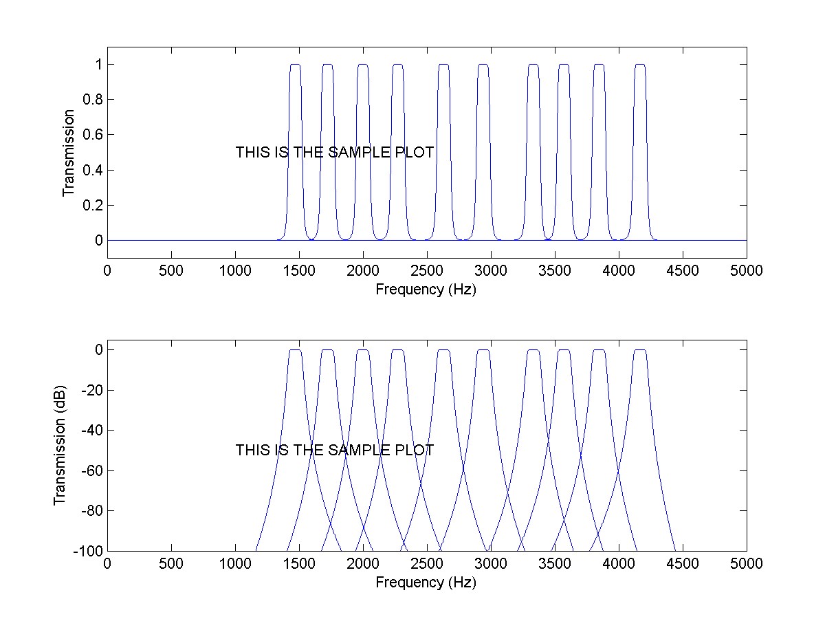
Plot the output of freqz against your frequency axis f_axis. You should create a frequency domain plot for each of the bandpass filters and overlay them on the same plot. The result should look similar to the following.

The horizontal axis should be the frequency in Hz and cover the entire allowable frequency band (0<f<5kHz). The vertical axis should be the magnitude of the frequency response.
Time Domain Bandpass Filter Analysis
The bandpass filters will eventually be implemented in ‘C’ code for execution on the laser tag system in the time domain. This reduces the computational cost of determining a hit to a level realizable on an embedded system. MATLAB will not be available on the laser tag system. However, we can model and simulate the signal processing system in MATLAB to make sure it will function as needed in the laser tag embedded system.
For this milestone, we need to analyze the output of each filter in the time domain and determine whether a hit was registered. The basic steps are the following:
- Create a square wave signal
- Use one of the player frequencies
- Sampling frequency Fs = 10 ksamples/s
- Pulse length of 200ms (2000 samples)
- Filter the square wave signal
- Pass the signal through each of the 10 bandpass filters
- Compute the total energy in each filtered signal
- Square and then sum each sample in the signal
- Plot the 10 energies
- Visualize if a ‘hit’ came through on a matching frequency
- Repeat the process for the next player frequency
Let’s walk through this process for the first player.
Step 1: Create a square wave signal
Use the MATLAB square function to create the signal. The square function is similar to the sin function except that it produces a square wave rather than a sine wave. Here is the MATLAB code to create the square wave:
Fs = 10e3;                   % The sampling frequency
t = linspace(0, 0.2, 2000);  % The time vector with a length of 0.2 seconds and 2000 total samples
freq = 1250;                 % The frequency of player 1
x = square(2*pi*freq*t);     % Create the time domain square wave
Step 2: Filter the square wave signal
Since our IIR filter coefficients are in SOS form, use the MATLAB sosfilt function to perform the actual filtering in this milestone. We need to filter the square wave signal (called ‘x’ in Step 1) using each of our 10 bandpass filters.
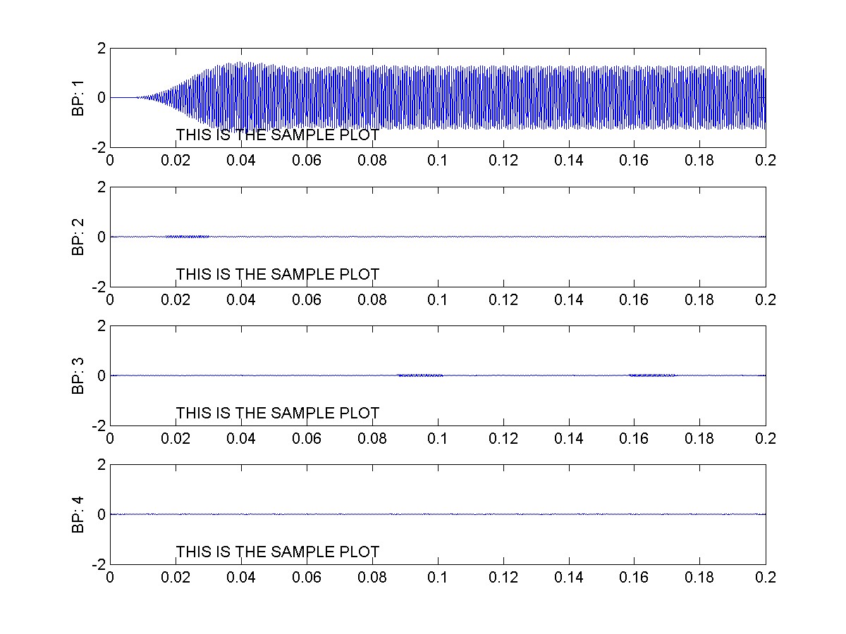
Plot the output of the filter function (operating on your square wave signal) for each of the 10 bandpass filters. The following plot shows the output of the first 4 bandpass filters when the square wave input has a frequency of 1250 Hz (player 1):

You can see from this plot that filters 2, 3, and 4 attenuate the signal a lot compared to filter 1 (look at the amplitudes of each filtered signal). The output of filter 1 has a much higher amplitude. If you zoom in on the output of filter 1 you should be able to see that the square wave was changed into a sine wave by the filter. (Do you understand why this happens? Remember that the square wave signal contains a sinusoid at the fundamental frequency, as well as higher frequency harmonics that give it a square shape. Our bandpass filter effectively takes out the higher harmonic frequencies that make it a square wave, leaving only the sinusoid at the fundamental frequency!)
Step 3: Compute the energy in each filtered signal
Looking at the outputs of the 10 filters, it is evident that when the square wave has a frequency that matches the frequency of a filter, the amplitude of the filtered signal will be much higher. You need a way of robustly determining which filtered signal has the highest average amplitude. However, if you simply take the largest value in each filtered signal, the system will be very susceptible to noise. A better way is to determine the total energy in each signal.
The total energy in a signal is found by squaring each sample over a window of time and then summing all of the squared samples. In our implementation, we are looking at a 200ms window of samples because that is the duration of our shots. These 200ms windows of output from each filter are sampled at 10 ksamples/s, yielding 2000 total samples. Thus, the summation for our signal energy calculation is only going to be over 2000 samples.
After we have computed the energy of each filtered signal, we can collect the results in an array.
Step 4: Plot the 10 energies
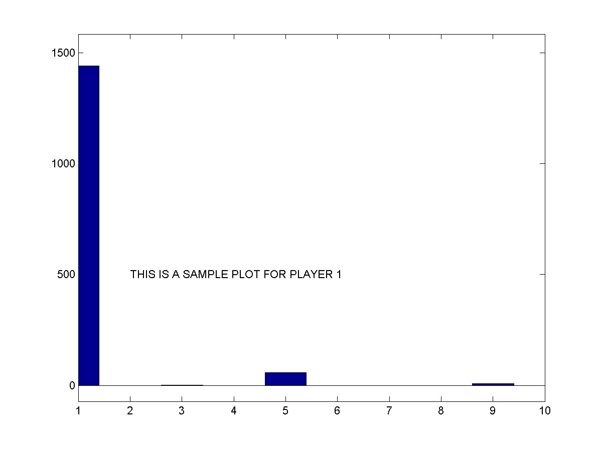
Next, plot a bar graph using the MATLAB bar function showing each of the energy array values. Your resulting bar graph, based on the player 1 signal, should look like this:

You should produce 10 of these plots, one for each of the 10 player frequencies. I suggest using the MATLAB tiledlayout function to tile small versions of each plot in a single figure. Visualize if a ‘hit’ came through on matching frequencies.
What is Needed in the Lab Report
- Description of your IIR bandpass filters
- Filter coefficients in SOS form (no more than 4 significant digits needed for report)
- Plots of the frequency response of your filters (using freqz)
- Description of the key components of the plots
- Analysis of the filtered signals
- Description of the energy calculation and its output window
- Bar graph plots of the total energy through each filter
- Description of the pertinent features of the plots
- Brief summary (1 paragraph) of what was accomplished
Pass Off
The following items need to be shown to the TAs for pass off:
- List (.csv file) of IIR filter coefficients in SOS form (with at least 7 significant digits) for each of the 10 bandpass filters
- Frequency response plot of the 10 filters overlaid in both linear and decibel scales
- Plots of the total energy resulting from a 200 ms duration square wave passed through each filter (There should be 10 of these plots corresponding to a square wave for each of the player frequencies.)