Design Lowpass Anti-Aliasing Filter
Table of contents
- Overview
- General Requirements
- General Notes
- Specifications
- Resources
- Actual Filter Design
- What is Needed in the Lab Report
- Pass Off
Overview
In this task, you will design the first stage of the laser tag signal processing system that takes a sampled signal from a photo diode, applies a lowpass filter to it, and then downsamples it to a lower sample rate. In the next stage, the signal is fed into a bank of 10 IIR filters to determine if there is a hit.
You will also be performing a noise analysis in this task. You will look at the spectrum of optical background noise sampled in a lab room at frequencies up to 40 kHz (the range that you can see using the data sampled at the full 80 ksamples/s), and then see how this noise aliases into the range from 1 to 5 kHz during the downsampling operation (when we downsample to 10 ksamples/s).
You will first try straight downsampling of the noise signal from 80 kHz to 10 kHz (just taking every 8th sample). You will see that you get severe aliasing using this process. You will then design a digital FIR anti-aliasing filter as part of your downsampling system to minimize high-frequency noise aliasing into the low-frequency bands (< 5 kHz) that we care about. The process of digitally filtering the signal first and then downsampling (by taking every 8th sample of the filtered signal in this case) is called “decimation”.
General Requirements
- Review aliasing and FIR filter design
- Demonstrate aliasing of actual optical noise during the downsampling process when no digital anti-aliasing filter is used
- Design a digital FIR lowpass anti-aliasing filter
- Analyze the performance of the FIR lowpass filter and see how it reduces noise aliasing in the downsampled signal
General Notes
For the noise analysis, you will use a previously measured time-domain signal of optical noise in a lab room. This signal is 500ms (half second) in duration and sampled at a rate of 80 ksamples/s, yielding a total of 40,000 samples. In this case, we simply want an optical noise signal without any player frequency signal on top of it. While you could acquire your own from the test setup in the lab, I suggest you use the provided optical noise signal light_80kHz.mat, since it is known to have sufficient noise to be detectable in this lab.
Specifications
Anti-aliasing FIR filter design specifications (we will discuss these more below):
- Maximum filter length: 81
- Maximum player variation: 1dB
- Corner frequency: between 4.5kHz and 5.5kHz
- Stopband: 10kHz < f < 40kHz
- Out of band rejection: 40 dB for frequencies between 10 and 40 kHz (also pay attention to attenuation in 5-10 kHz range, but doesn’t need to meet the 40 dB rejection there)
- Player frequencies: 1250, 1481, 1739, 2000, 2353, 2667, 3077, 3333, 3636, 4000 (all in Hz)
Resources
Optical Noise Sample
- Time-domain signal of optical noise: light_80kHz.mat
- Sampling Frequency: 80 kHz
- Duration: 500ms
- Format: MATLAB file (.mat) for storing workspace variables
- Contains two array variables, y and t
- y: single-precision data with an amplitude of 1
- t: time stamp of each sample in seconds
Use the MATLAB load command to read in the data.
load light_80kHz % read optical noise data
MATLAB fft Help
A clear description of how to use the MATLAB fft function to display the single-sided amplitude spectrum can be found in the MATLAB fft documentation. Once you have clicked the link, scroll down to the “Single-Sided Amplitude Spectrum” example. More fft usage examples can be found on this page.
Aliasing Background
To start off, you should review aliasing with sampled signals. You covered this in ECEN 380. You can also read about it online on Wikipedia.
As you know, it is hard to see the aliasing problem by looking at a time domain plot. However, in ECEN 380 you learned about looking at signals in the frequency domain. We are again going to use the MATLAB fft function for performing the fast Fourier transform (FFT) on your signal data.
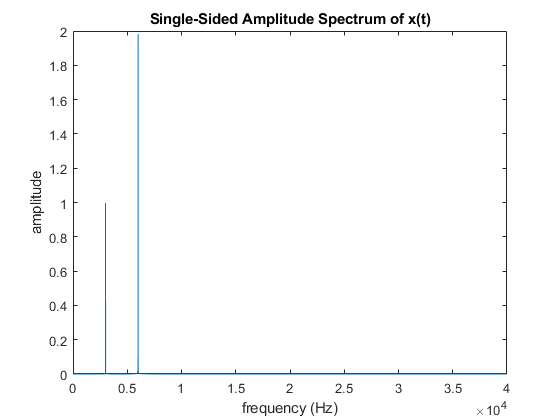
Let’s explore aliasing using some synthesized data. In MATLAB, you are going to generate two sine waves, one with a frequency of f1 = 3 kHz and amplitude of A1 = 1 V, and one with a frequency of f2 = 6 kHz and amplitude of A2 = 2 V. The MATLAB code to produce these signals (using an 80 kHz sample rate) is:
Fs = 80e3;  % sample rate
f1 = 3e3;   % signal frequency
f2 = 6e3;
A1 = 1;     % signal amplitude, this is peak amplitude not peak-to-peak
A2 = 2;
% We're going to use a time axis from -0.25 to 0.25 seconds, which is 0.5s wide
% This yields Fs*0.5s total samples on our time axis
t = linspace(-0.25, 0.25, Fs*0.5);
x = A1*sin(2*pi*f1*t) + A2*sin(2*pi*f2*t);
Use the MATLAB fft function to produce the Fourier transform of your signal. Your signal should look like the image shown below (if you only plot the positive frequency axis after doing the FFT). Zoom in on the spikes and make sure that they are centered at 3 kHz and 6 kHz. If your signal does not look like this plot then you might want to go back and review the MATLAB fft function.
Now you are going to downsample the data to a sampling frequency of Fs = 10 kHz. We will accomplish this by taking every eighth sample of the original signal. Here is MATLAB code to perform the downsampling:
x_ds = x(1:8:length(x));
t_ds = t(1:8:length(t));
Fs_ds = Fs/8;
Since the new sample rate is 10 kHz, the maximum frequency we can resolve is now reduced to 5 kHz. The 3 kHz sine wave is below 5 kHz, so we would expect that frequency to remain unchanged in the downsampled signal. However, we would expect the 6 kHz signal to produce aliasing at 4 kHz with the new sample rate. (Do you understand why?)
Use the MATLAB fft function to calculate the frequency domain plot of your new downsampled signal. You should produce a plot that looks something like this:
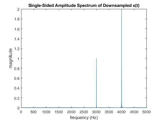
Again, you can see the formerly 6 kHz signal aliasing into the new frequency range as a 4 kHz signal.
What would happen if the second sine wave originally had a frequency of 7 kHz instead of 6 kHz? (Answer: It would alias down to 3 kHz, on top of the original 3 kHz signal!)
Aliasing of Noise
The performance of the laser tag system can be improved by reducing the noise that ultimately ends up across the band of frequencies we care about (~1 - 5 kHz). We are not going to be investigating all of the noise sources in our system, but we are going to look into one of the easiest noise sources to reduce: the optical noise produced by the lights in our lab room.
We measured the signal produced by the lights in the lab and saved it as a MATLAB file (light_80kHz.mat). This data is all noise. You can load it directly into MATLAB. It contains two variables, y and t. (Use the MATLAB load command.)
You should get a plot similar to the following:
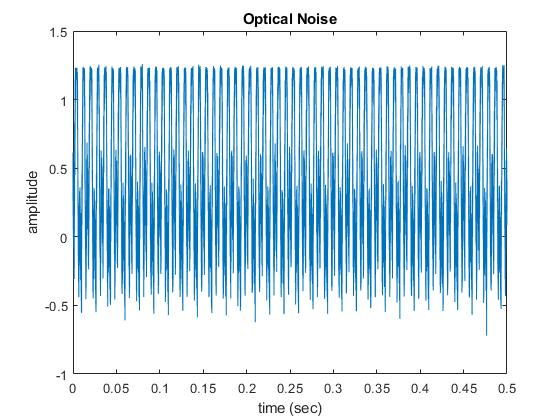
As mentioned, this signal is all noise. It is hard to imagine the ability to detect a signal with an amplitude of ~10mV if the noise has an amplitude of ~1000 mV. That is the beauty of signal processing. To be able to understand this noise signal, we need to plot it in the frequency domain.
As we’ve now done many times before, you can plot the signal in the frequency domain using the MATLAB fft function. As you know, in order to get the frequency axis right after performing the FFT you need to know the sampling frequency of the data. If you didn’t happen to know the sampling frequency of this data, you could extract it from the time vector by looking at the difference between subsequent time data points (which would be the sampling period, or 1/Fs).
Fs=1/max(diff(t))
Produce a frequency domain plot of the noise you loaded from the file provided. It should look something like the following:
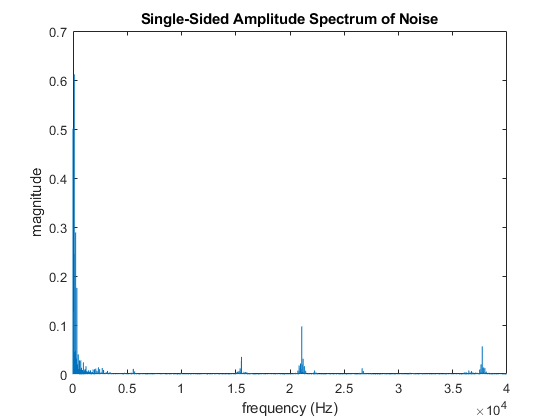
This plot shows that the noise is clumped around three main locations (1) low frequencies, (2) near 21 kHz, and near 38 kHz.
Zoom in on the plot and note the amplitude of the frequency components in the band where our player frequencies are located (1kHz < f < 5 kHz).
Now, as we discussed in lab lecture, the laser tag system sampling frequency is 80 kHz. However, the 10 bandpass filters to be designed in Milestone 2 Task 2 are to have a sample rate of 10 kHz (since we only care about signals < 5 kHz and we want to keep our computations simple so our filtering can be done in real time on the laser tag system). That means we need to downsample the data to a 10 kHz sample rate.
Let’s first try getting to the new lower sample rate by simply using every eighth sample like we did before when we reviewed aliasing. Downsample your measured signal (which is 40,000 samples long, sampled at 80 kHz) to a 5,000 sample signal by taking every eighth sample.
Plot the downsampled signal in both the time domain and frequency domain. It should look similar to the following:
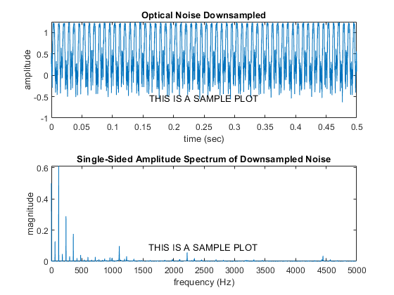
Notice that the time domain signal looks very similar. However, the frequency domain signal now has a maximum frequency of 5 kHz (i.e., half of your new sampling frequency of 10 kHz). The noise in our desired frequency band (1kHz < f < 5kHz) is now drastically higher than it was prior to downsampling. This increase in the noise is caused by aliasing of some of the higher frequency peaks in the original signal (in our noise data, there is a peak at f = 21 kHz and f = 38 kHz that alias into the band we are interested in).
So how can we avoid getting all of this higher-frequency optical noise aliasing into our 1 - 5 kHz band when we downsample to 10 kHz?
The solution is to use a digital lowpass anti-aliasing filter before we downsample the data. If we want to downsample the data to a new sampling frequency of 10 kHz, our digital anti-aliasing filter would ideally have a cut-off frequency of 5 kHz. It would then filter out the higher frequency noise (like the 21 kHz and 38 kHz peaks we saw in our data) before we take every eighth sample, avoiding the aliasing problem. This process of first digitally filtering our signal (sampled at a high sample rate) and then downsampling the filtered signal is called ‘decimation’.
So to summarize, what our system is going to do is (1) sample the incoming data at a sample rate of 80 kHz, (2) filter our higher frequencies from this data using a digital lowpass anti-aliasing filter, (3) downsample the filtered data to a sample rate of 10 kHz, and (4) send the resulting signal through our bank of 10 filters to determine if there is a player hit.
Anti-Aliasing Filter Design
Your next task is to design the digital anti-aliasing filter discussed above.
There is a very clever trick that we can use to reduce the computational complexity of this decimation step (digital filtering followed by downsampling). If we use an FIR filter (refer back to the Discrete-Time Filters Lab material from ECEN 380 for a review of FIR filter design), then the digital filtering step can be performed with a discrete finite convolution in the time domain. The convolution involves performing a sum for each of the samples in the output signal. However, after the digital filtering operation, we are going to throw away 7 out of every 8 samples in the resulting signal anyway. So why bother computing those 7 values that we are going to throw away? If we only compute the 1 out of 8 values that we need, we will cut the operations needed to perform our filtering down by a factor of 8. See decimating for more information.
When we actually implement real-time decimation on our laser tag system, that’s exactly what we’ll do. For now, however, let’s design our FIR filter, determine the filter coefficients, and then simply use the MATLAB filter function, followed by downsampling. This will be perfectly adequate for testing our signal processing algorithms before we implement them on the laser tag system.
The specifications of the filter are provided at the top of this page. You will be using the FIR filter design process that you used in ECEN 380. For your convenience, here is a link to the ECEN 380 Discrete-Time Filters Lab.
To refresh your memory, the basic process is:
- Consider a rect function in the frequency domain with the appropriate width
- Determine the resulting sinc function in the time domain
- Multiply the time-domain sinc function times a windowing function (to limit the length of the impulse response, and to reduce the height of the side lobes in the frequency response of the filter)
The main design parameters of the filter are the following:
- Filter length
- Corner frequency
- Filter windowing
Filter Characterization
Two MATLAB functions useful for characterizing a filter are the following:
To understand how this works we are going to look at a filter with a windowing function. (In your design you will be adding in a windowing function.) Let’s look at a lowpass filter with a corner frequency of f = 5 kHz. In the frequency domain this would be a rect function. If you take the inverse Fourier transform of a rect function you get a sinc function. The length of the filter determines how much the filter looks like the ideal sinc function.
Let’s start by looking at the filter in the time domain. (This means that we are looking at the impulse response of the filter.) Since we are working with data sampled at a frequency of 80 kHz, the maximum frequency we can resolve is Fs/2 = 40 kHz.
When you review your ECEN 380 code for designing digital filters, you may be confused by seeing frequencies described in a variety of different units. In this lab, we are dealing with time domain signals, and a natural way to think about frequency is in units of cycles/s, or Hertz. However, you may see frequencies in your FIR filter design code from ECEN 380 in units of cycles/sample. These units are often used in digital filter design. To convert from frequency in Hz to frequency in cycles/sample, do the following:
(Frequency in cycles/sample) = (Frequency in Hz) / (Sampling frequency)
Furthermore, you will sometimes see frequencies in units of radians/sample. To convert from frequency in cycles/sample to frequency in radians/sample, do the following:
(Frequency in radians/sample) = 2*pi*(Frequency in cycles/sample)
Occasionally, certain MATLAB functions will use other units, like half-cycles/sample (where a frequency of 1 corresponds to one-half the sampling frequency).
The important thing to take away from all of this is to be consistent in what units of frequency you are using. Also, make sure to read the help for each MATLAB function that requires frequencies to ensure that you are passing in frequencies in the units that the MATLAB function is expecting. And remember that certain MATLAB functions (like freqz) have several different forms depending on what parameters you pass in, and that those different forms might require frequencies in different units. For example, here is the MATLAB help descriptions from two of the different forms of freqz:
H = freqz(B,A,W) returns the frequency response at frequencies
    designated in vector W, in radians/sample (normally between 0 and pi).
    W must be a vector with at least two elements.

H = freqz(B,A,F,Fs) returns the complex frequency response at the
    frequencies designated in vector F (in Hz), where Fs is the sampling
    frequency (in Hz).
The first form of freqz above takes the input frequencies in radians/sample, whereas the second form takes the input frequencies in Hz (and then requires a sampling frequency so that it can convert for you.)
With this in mind, a lowpass filter with a corner frequency of 5 kHz that operates on data sampled at 80 kHz would be a rect function that goes from -0.0625 to 0.0625 in cycles/sample. (Can you see why? We want the lowpass filter to go from -5 kHz to 5 kHz, and the data was sampled at Fs = 80 kHz. So, in units of cycles/sample, our rect goes from -5kHz/80kHz = -0.0625 to 5kHz/80kHz = 0.0625 cycles/sample.)
The FIR filter can be realized with the following MATLAB code:
N = 201;      % filter length
L2 = (N-1)/2; % the filter will go from –L to L
n = (-L2:L2); % this is our filter index

f_corner = 5000; % corner frequency of our lowpass filter in Hz
f_s = 80000;     % our sampling frequency in Hz

% IMPORTANT: in the line below, we convert f_corner from Hz
% to cycles/sample by dividing by f_s
h = 2*f_corner/f_s*sinc(n*2*f_corner/f_s); % sinc function
h1 = h .* hamming(N).'; % apply Hamming window
FIR_b = single(h1); % convert to 32-bit (single) precision
The laser tag system only has single precision (32-bit) floating-point hardware. Therefore, make sure that your MATLAB filter coefficients and sample data are in single precision so that your modeling and simulation results are representative of how it will run on the laser tag system. MATLAB defaults to using double precision (64-bit) floating point, so the use of single is needed to convert filter coefficient variables to single precision.
Plot the resulting windowed sinc function for both a long (N = 201) and short (N = 21) filter length. Your resulting plots should look like the following:
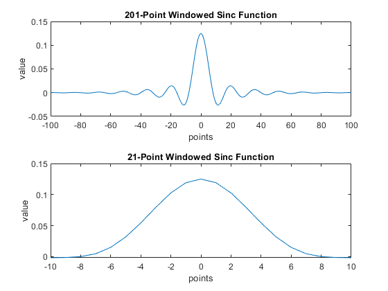
Notice how the longer filter looks a lot more like the sinc function than the shorter one.
Now we want to look at the resulting filters in the frequency domain. We are going to do this by using the freqz MATLAB function. The freqz MATLAB function is used for both FIR and IIR digital filters. Since we just designed an FIR filter, our impulse response (time domain) directly gives the b coefficients of our filter. The a coefficients are a0 = 1 and a1, a2, … = 0. (If this isn’t sounding familiar, review the FIR filter design section of the ECEN 380 Discrete-Time Filters Lab.)
Use the freqz function to plot the frequency response of your N = 201 and N = 21 length filters. Your plots should look like the following:
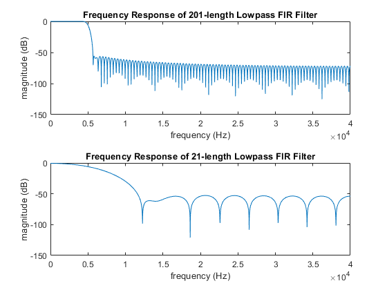
Notice that the long filter looks a lot more like your desired lowpass filter.
Now let’s look at how we specify the performance of a filter. This picture illustrates the various regions of a lowpass filter:
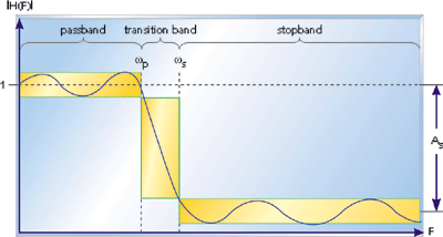
The ideal lowpass filter has a flat frequency response in the passband region, complete attenuation in the stopband region, and an infinitely thin transition band.
We have 1 specification related to the passband region and 1 related to the stop band region.
Specification 1 (We call this Player Variation): This specification is similar to what is called Passband Ripple. Passband Ripple is the total variation in the frequency response for frequencies within the passband. However, our specification is a little bit looser than Passband Ripple. We just want to make sure that the filter has the same response for each player. So our specification is the total variation in the response for the 10 player frequencies.
Specification 2 (This one is called Out of Band Rejection): This specification is the amount of attenuation experienced by any signal with a frequency component within the stopband. Since we are designing a lowpass filter, the stopband is any frequency larger than the transition band.
Player Variation
This specification is related to changes to the player signals. If one player signal is being attenuated more than another by the filter, then that player will have an advantage because the player shooting will need to be closer. Therefore, a system with a lot of player variation would be a poorly designed game.
To determine Player Variation, we plug each of the player frequencies into the transfer function of our lowpass FIR filter and see what the gain is at each of the 10 player frequencies. We then take the ratio of the smallest value to the largest value (typically reported in decibels, so 20*log10(ratio of smallest player gain to largest player gain)).
The easiest way to find out what the gain is at each of the 10 player frequencies is to pass freqz a vector with the 10 player frequencies, and it will return the gain at each frequency.
- For the long (N = 201) filter
- The values are: 0.99991, 1.00043, 0.99971, 0.99979, 1.00043, 0.99925, 1.00084, 0.99934, 0.99988, 1.00101
- This corresponds to a variation of 0.99925/1.00101=0.99825. As mentioned, we’ll typically report this in decibels instead. So this variation becomes 20*log10(0.99825)=-0.01523 dB, which meets the specification because -0.01523 > -1
- For the short (N = 21) filter
- The values are: 0.90002, 0.88721, 0.87051, 0.85115, 0.82123, 0.79126, 0.74786, 0.71858, 0.68208, 0.63602
- This corresponds to a variation of 0.63602/0.90002=0.70666. So this variation becomes 20*log10(0.70666)=-3.01574, which does not meet the specification because -3.01574 < -1
Out of Band Rejection
The objective of the anti-aliasing filter is to attenuate any signals with frequency components above about 5 kHz (i.e., half the final sample rate). The distance between the highest player frequency (4000 Hz) and the maximum frequency (Fs/2 = 5 kHz) is 1000 Hz. This would make the transition band 4000Hz < f < 6000Hz.
This transition band is fairly small, which would make the design of the lowpass filter difficult. Therefore, we are going to widen the transition band to make the design easier. We are going to use a transition band of 4.5kHz < f < 10kHz.
This wider transition band means that some noise within the transition band can alias into our passband. However, we fortunately don’t have much optical noise in these frequency bands, as shown here:
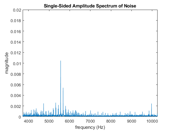
You can see that the noise is fairly low in the transition band, so our looser specification should not result in too much additional noise aliasing, and shouldn’t have too much impact on our final signal.
To evaluate this specification (Out of Band Rejection), use the freqz function again, but this time pass in a frequency array with values from 10 kHz up to 40 kHz. This will return the frequency response across the range of frequencies in your stop band. The maximum gain (absolute value of your frequency response) across this range of frequencies is your Out of Band Rejection. Similar to the Player Variation specification, you should also report this maximum gain in units of decibels. However, unlike Player Variation, in this case we want the number to be as small as possible.
For the long filter length, Out of Band Rejection should be around -62 dB, and for the short one it should be around -30 dB.
Actual Filter Design
You have now done a simple filter design, plotted the response of the filter in the time domain and frequency domain, and determined the specifications of a filter. You are now ready to design and characterize the lowpass FIR filter that you are actually going to use.
In the sections above, we were able to get an FIR filter to meet all of the performance specifications. However, the filter is too long. With a filter length of 201, you will use up too much of the processing power of the laser tag system.
We are limiting you to an FIR anti-aliasing filter length of 81. To meet the performance specs with this length of a filter, you will need to optimize the windowing function, and possibly use a corner frequency higher than 5 kHz.
As a review here are the design parameters.
- Filter length (limited to a length of 81)
- Windowing function
- Corner frequency
Happy filter designing, and good luck! :-)
Noise Reduction
Now that you have finished the design of the anti-aliasing filter, your final job is to see how well it reduces the aliased noise. Do the following:
- Load in the optical noise sample (light_80kHz.mat), which is 500ms long with 40,000 samples)
- Plot the noise spectrum (frequency domain) without using your FIR filter (like you did before)
- Downsample to Fs = 10kHz
- Plot the noise from 1kHz to 5 kHz
- Plot the noise spectrum (frequency domain) using your FIR filter
- Filter the noise signal with your FIR filter before downsampling
- Downsample the signal to Fs = 10kHz
- Plot the noise from 1kHz to 5 kHz
- Compare the two signals
Hopefully you are getting pretty comfortable with this kind of MATLAB coding at this point, but here is some example code if you need some help:
% Clear command window & workspace, and close all figures
clc, clear, close all;

load light_80kHz % read optical noise data

% downsample
y1 = y(1:8:length(y));
t1 = t(1:8:length(t));
Fs = 1/max(diff(t1)); % sampling frequency, which should be 10 kHz

% calculate frequency spectrum
Y1 = fft(y1);
len = length(Y1);
Y1 = Y1(1:floor((len)/2));
Y1 = 2*Y1/len;
freq = linspace(0, Fs/2, length(Y1));

% copy your filter coefficients here
b = [  ];

y2 = filter(b,1,y); % filter the optical noise using the FIR filter

% downsample
y3 = y2(1:8:length(y2));

% frequency spectrum
Y3 = fft(y3);
len = length(Y3);
Y3 = Y3(1:floor((len)/2));
Y3 = 2*Y3/len;

% plot the 2 noise spectra
figure;
tiledlayout('vertical');

nexttile;
plot(freq*1e-3,abs(Y1));
title('Raw Noise');
xlabel('frequency (kHz)');
ylabel('magnitude');
ylim([0 .2]);

nexttile;
plot(freq*1e-3,abs(Y3));
title('Filtered Noise');
xlabel('frequency (kHz)');
ylabel('magnitude');
ylim([0 .2]);
Save Coefficients
Make sure to save your FIR filter coefficients for a later lab as a .mat file. Also, save them in a human readable format (.csv file) for your report and pass-off. The following code assumes your filter coefficients are stored in the MATLAB variable FIR_b.
% save FIR filter coefficients
save("FIR_b.mat","FIR_b");
writematrix(FIR_b,'FIR_b.csv','WriteMode','overwrite');
In a future milestone, you will need to convert your MATLAB filter coefficients into ‘C’ code for the laser tag system. A script will be provided to ease this conversion. The script expects the following naming convention and format for the FIR filter coefficients when saved to a .mat file:
- FIR_b is a 1 x N vector of single-precision floating-point values
- N is the length of the filter (81)
What is Needed in the Lab Report
- Description demonstrating an understanding of aliasing (include MATLAB plots that you generated)
- Description of your FIR lowpass filter design
- Bandwidth and windowing details
- Filter coefficients (no more than 4 significant digits needed for report)
- Achieved filter specifications (give numbers for player variation, out-of-band rejection)
- Frequency response plot (i.e., transfer function of the filter)
- Optical Noise
- Plot of optical noise downsampled to Fs = 10 kHz (just taking every 8th sample)
- Plot of optical noise decimated to Fs = 10 kHz (lowpass filtered + downsampled)
- Brief summary (1 paragraph) of what was accomplished
Pass Off
The following items need to be shown to the TAs for pass off:
- MATLAB code segment showing design of FIR lowpass anti-aliasing filter
- List (.csv file) of FIR filter coefficients (single precision with at least 7 significant digits)
- List of achieved filter specifications (show numbers for player variation, out-of-band rejection)
- Frequency response plot of the lowpass FIR filter
- Plot of optical noise doing a straight downsampling to 10 kHz (with no FIR filter)
- Plot of optical noise decimated to 10 kHz (lowpass filter + downsampled)