MATLAB Help
Table of contents
Basic Functions
- len
- plot
- subplot
- hold
- sin
- square
- xlim
- ylim
You can type help <name> to get a description of the particular function.
Let’s do an example to use these basic functions. We are going to plot 4 different signals on 2 separate plots.
- Plot 1 will contain a square wave and sine waves with amplitude of 2 and frequency of f=1 kHz.
- Plot 2 will contain a square wave and sine waves with amplitude of 2 and frequency of f=10 kHz.
Here is the MATLAB code for the first plot.
f1 = 1e3;
fs = 100e3;
t  = 0:1/fs:10/f1;
y1 = sin(2*pi*f1*t);
y2 = square(2*pi*f1*t);

subplot(2,1,1);
hold off;
plot(t*1e3,y1,'b');
hold on;
plot(t*1e3,y2,'r');
hold off;
ylabel('amplitude');
xlabel('time (ms)');
ylim([-1.2 1.2]);
Here is a description of the MATLAB code.
- We use a variable for the signal frequency (f1) and the sampling frequency (fs).
- We create a vector for the time (t). It has an increment of the sample period (1/fs) with a duration of 10 signal periods (10/f1).
- We create the vectors for the sine and square waves.
- We use the subplot function to plot the signals in the upper half of the plot window.
- The hold on makes it so that the next plot function call overlays onto the same plot. hold off does the opposite.
- Use xlabel and ylabel to add in axes.
The second part of the code is similar and just changes the frequency, the time, and the plot location. Here is the resulting MATLAB code.
f2 = 10e3;
t  = 0:1/fs:10/f2;
y3 = sin(2*pi*f2*t);
y4 = square(2*pi*f2*t);

subplot(2,1,2);
hold off;
plot(t*1e3,y3,'b');
hold on;
plot(t*1e3,y4,'r');
hold off;
ylabel('amplitude');
xlabel('time (ms)');
ylim([-1.2 1.2]);
The resulting plot should look like the following. 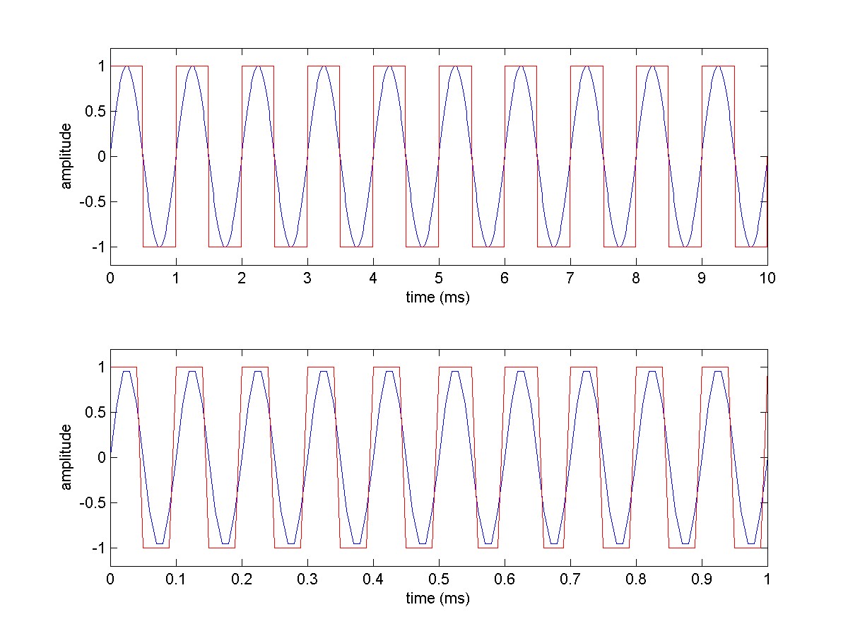
Filtering Function Help
- butter: Butterworth filter design
- filter: Time domain filtering of a signal
- fft: Fast Fourier Transform
- freqz: complex frequency response of a digital filter
butter
Start by typing
help butter
on the MATLAB command line. Read through the description. Let’s look at parts of the description and what it means.
Description: “butter Butterworth digital and analog filter design.”
Why we care: We are designing a digital filter so this should help.
Description: “[B,A] = butter(N,Wn) designs an Nth order lowpass digital Butterworth filter and returns the filter coefficients in length N+1 vectors B (numerator) and A (denominator).”
Why we care: The B (numerator) and A (denominator) coefficients means that it calculates the coefficients of an IIR filter (see IIR).
Description: “The cutoff frequency Wn must be 0.0 < Wn < 1.0, with 1.0 corresponding to half the sample rate.”
Why we care: When we design the cutoff frequencies we divide our desired cutoff frequency by half the sample rate to get it into the correct form for the butter function.
Description: “If Wn is a two-element vector, Wn = [W1 W2], butter returns an order 2N bandpass filter with passband W1 < W < W2.”
Why we care: Rather than simply designing a lowpass filter we can calculate the IIR filter coefficients for a bandpass filter, which is what we want.
filter
Type
help filter
on the MATLAB command line. Read through the description. Let’s look at parts of the description and what it means.
Description: “One-dimensional digital filter.”
Why we care: We want to do a one dimensional filter so it looks like we have the correct function.
Description: “Y = filter(B,A,X) filters the data in vector X with the filter described by vectors A and B to create the filtered data Y.”
Why we care: Our sampled data is the X vector and the resulting sampled data is the Y vector.
Description: “If a(1) is not equal to 1, filter normalizes the filter coefficients by a(1).”
Why we care: We need to make sure that the first element of our a vector is equal to 1.
fft
MATLAB has a function for performing numerical Fourier transforms called the fast Fourier transform (FFT). The FFT is actually a discrete Fourier transform (DFT). We can relate the DFT to the continuous time domain. This FFT video explains the conversion between the time and frequency domains. MATLAB also has some help on using the FFT. In the command window type
help fft
More detailed MATLAB fft documentation is available online.
freqz
Let’s go through the MATLAB help and find the portions that are the most pertinent. Start by typing
help freqz
Description: “freqz Frequency response of digital filter.”
Why we care: We want the frequency response of a digital filter. So it looks like we found the correct MATLAB function.
Description: “[H,W] = freqz(B,A,N) returns the N-point complex frequency response vector H and the N-point frequency vector W in radians/sample of the filter:”
Why we care: H is the complex frequency response. N is the number of points that are calculated.
We don’t really want the plot in terms of radians/sample. We would prefer to create the plot in terms of frequency. So we are going to scan down the description until we find the form of freqz that is in terms of frequency.
Description: “H = freqz(…,F,Fs) returns the complex frequency response at the frequencies designated in vector F (in Hz), where Fs is the sampling frequency (in Hz).”
Why we care: This tells us how to create the plot in terms of frequency rather than samples.
Filtering Function Examples
Using butter and filter
Let’s do a simple example to make sure that we understand how to use the butter and filter MATLAB functions.
We are going to start with a lowpass filter to make sure that we have the cutoff frequency set properly.
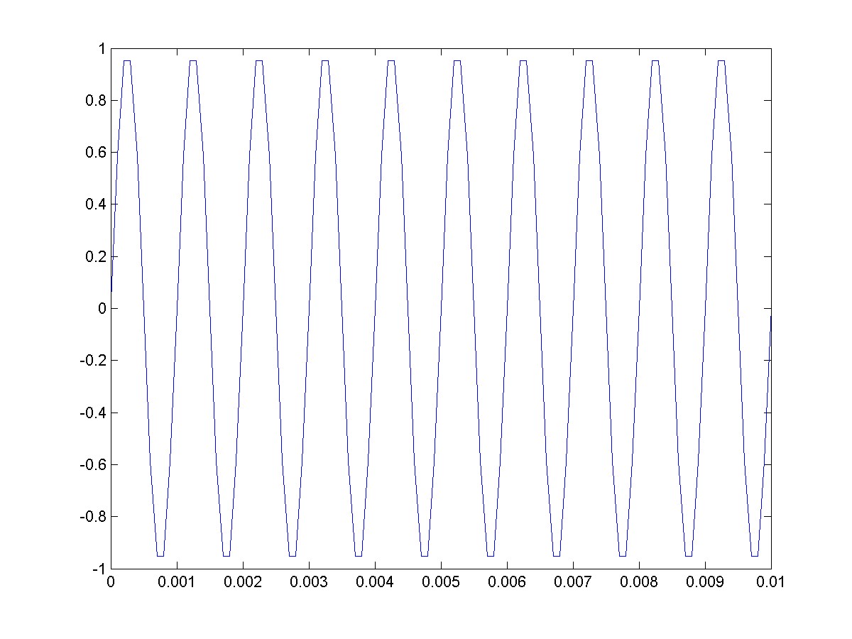
Plot a sinusoidal signal with a frequency of f1=1kHz, sampling frequency of Fs=10e3, and plot 10 periods of the signal.
Fs = 10e3;
f1 = 1e3;
t = 0:1/Fs:10/f1;
x1 = sin(2*pi*f1*t);
plot(t,x1);
You should get a plot that looks like:
If we create a lowpass filter with a cutoff frequency of fcut=1.5kHz then the signal should pass through the filter. Let’s make some mistakes and see what happens and see if we can figure out what we did wrong. We are doing this to learn about debugging.
Mistake: Pass the cutoff frequency as the actual frequency.
Wn = 1.5e3;
[B,A] = butter(5,Wn);
We get an error message that says “…cutoff frequencies must be within the interval of (0,1).” We would type help butter and find out that “Wn must be 0.0 < Wn < 1.0, with 1.0 corresponding to half the sample rate.”
Mistake: Divide the cutoff frequency by Fs rather than Fs/2.
Wn = 1.5e3;
Wn = Wn/(Fs);
[B,A] = butter(5,Wn);

y = filter(B,A,x1);

subplot(2,1,1);
plot(t,x1);
ylabel('original');

subplot(2,1,2);
plot(t,y);
ylabel('filtered');
The resulting plot should look something like:
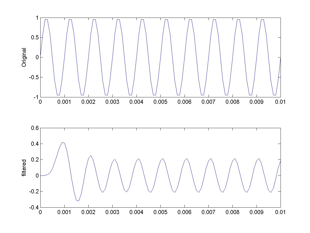
The signal y has a lower amplitude. This means that it is being filtered. We must have made an error in the cutoff frequency. If we make the following change
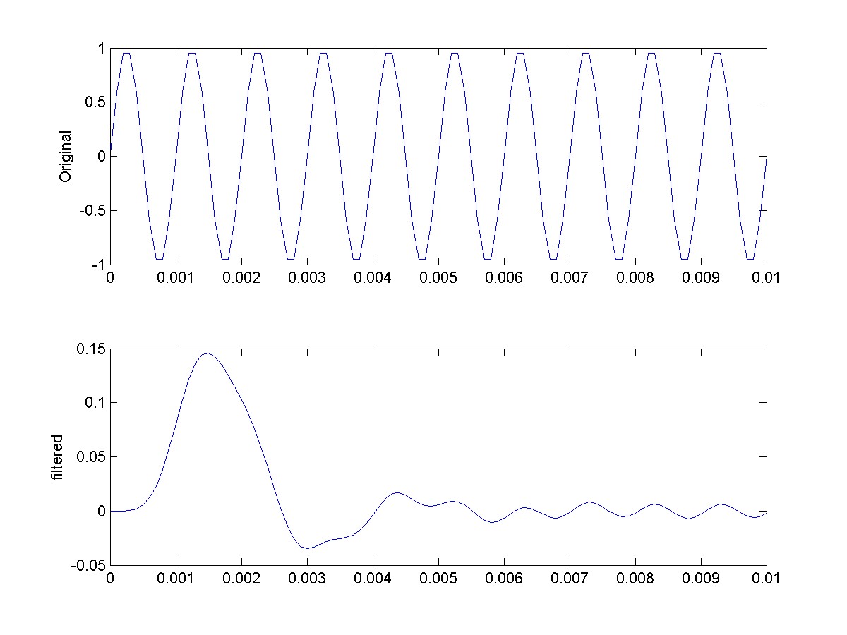
Wn = Wn/(2*Fs);
The following plot shows that it is now worse because we were supposed to divide by Fs/2 not 2*Fs.
The correct value is
Wn = Wn/(Fs/2);
Resulting in the correct plot.
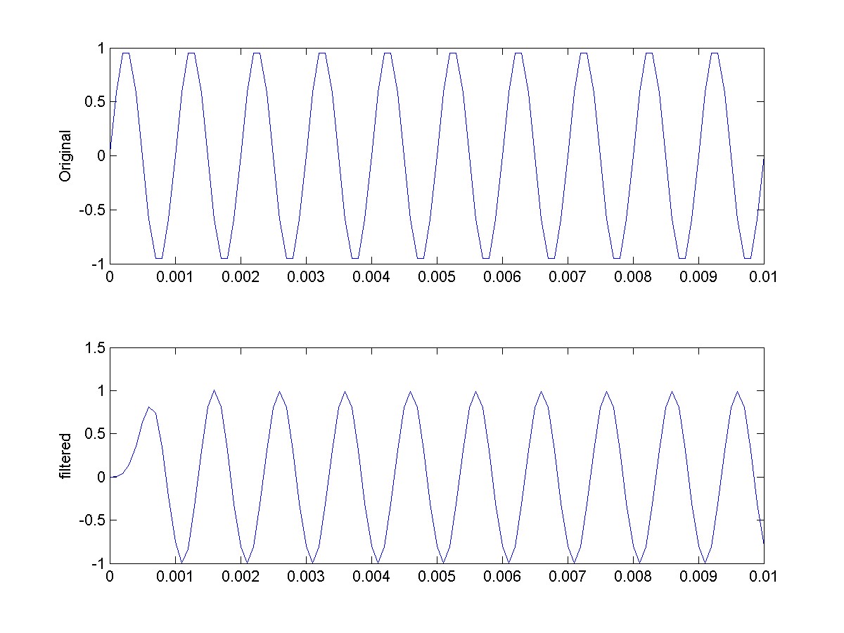
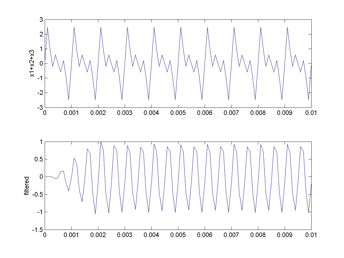
To finish up let’s make sure that we can use the butter function to create a bandpass filter. Start with a signal that is x=sin(2*pi*1e3*t)
- sin(2*pi*2e3*t) + sin(2*pi*3e3*t) and has the a sampling frequency of Fs=10kHz. Use a bandpass filter to pass the f=2kHz signal through and attenuate the other two. The resulting plots should look like the following.
Using fft
Let’s go through an example besides the one provided in the MATLAB help to make sure that you understand how to use the FFT.
You need to create a frequency domain plot of a sinusoidal signal with frequency of f1=3 kHz and amplitude of 1. We are using a sinusoidal signal because we know that the Fourier transform of a sine wave is a delta function. So the FFT should produce a spike at a frequency of 3 kHz and have an amplitude of 1.
Here is the MATLAB code to create the time signal
Fs = 100e3; % sample rate
f1 = 3e3;   % signal frequency
A1 = 1;     % signal amplitude, peak amplitude not peak-to-peak
t  = 0 : 1/Fs : 10/f1;
y  = A1*sin(2*pi*f1*t);
Here is the plot of our signal.
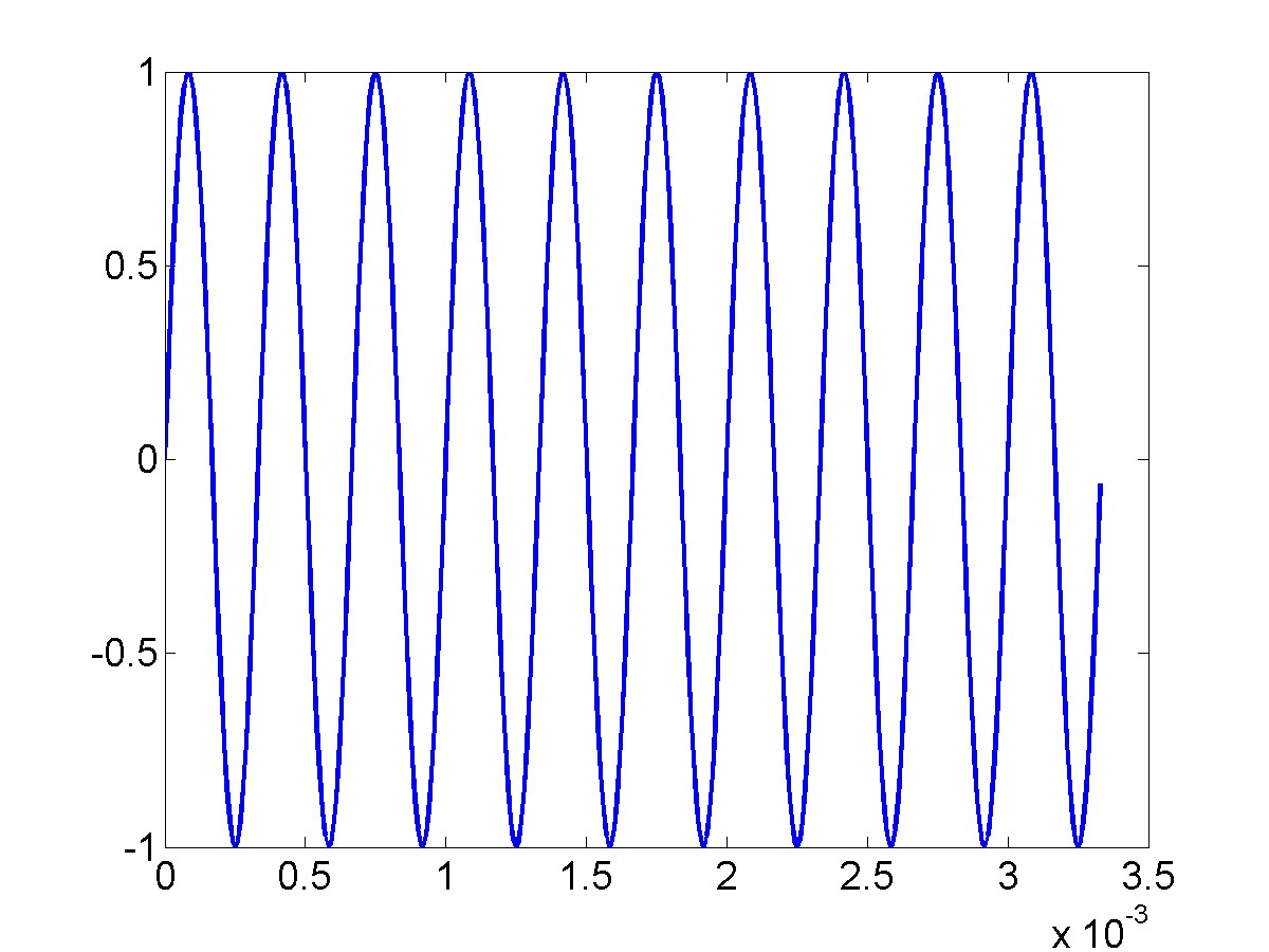
Now you need to create the Fourier transform of the signal using the MATLAB fft function.
Y = fft(y);
plot(abs(Y));
Notice that we plotted the absolute value of Y since it is complex.
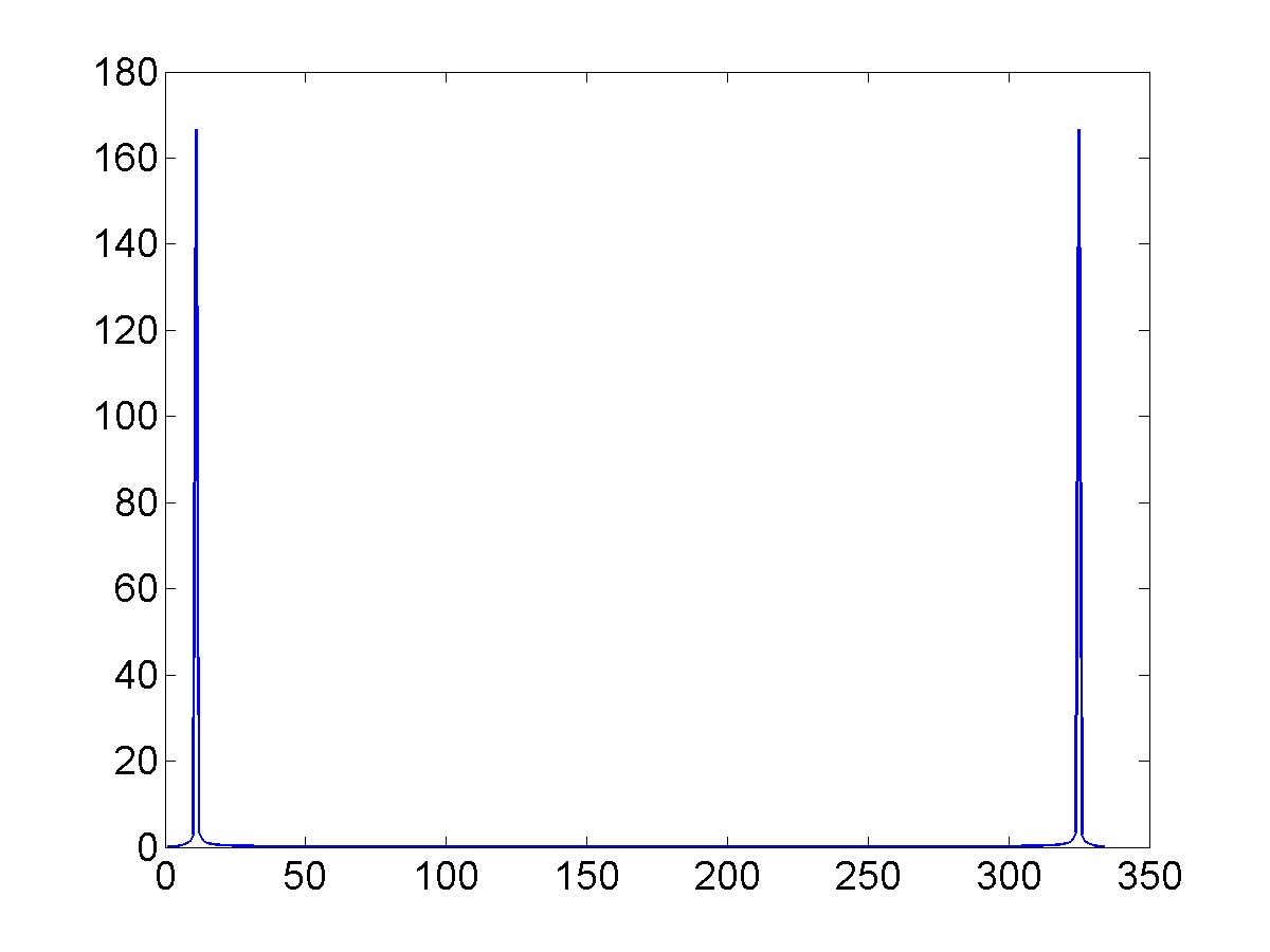
Notice that there are two spikes and that the amplitude is not equal to our amplitude of 1.
Let’s start with the frequency. We only want the positive frequencies so we are only going to use the first half of the vector. We know that maximum frequency of a sampled signal is Fs/2. So we create an x-axis vector that goes from 0 to Fs/2 and has a length of half of Y. Here is the resulting MATLAB code.
L  = length(Y);            % the total length of our fft
Y1 = Y(1:L/2);             % take the first half of the vector
f  = linspace(0,Fs/2,L/2); % create the frequency vector
plot(f,abs(Y1));
The linspace function creates a vector with equally spaced elements between a starting and an ending value and with a specified number of elements. Here is the resulting plot.
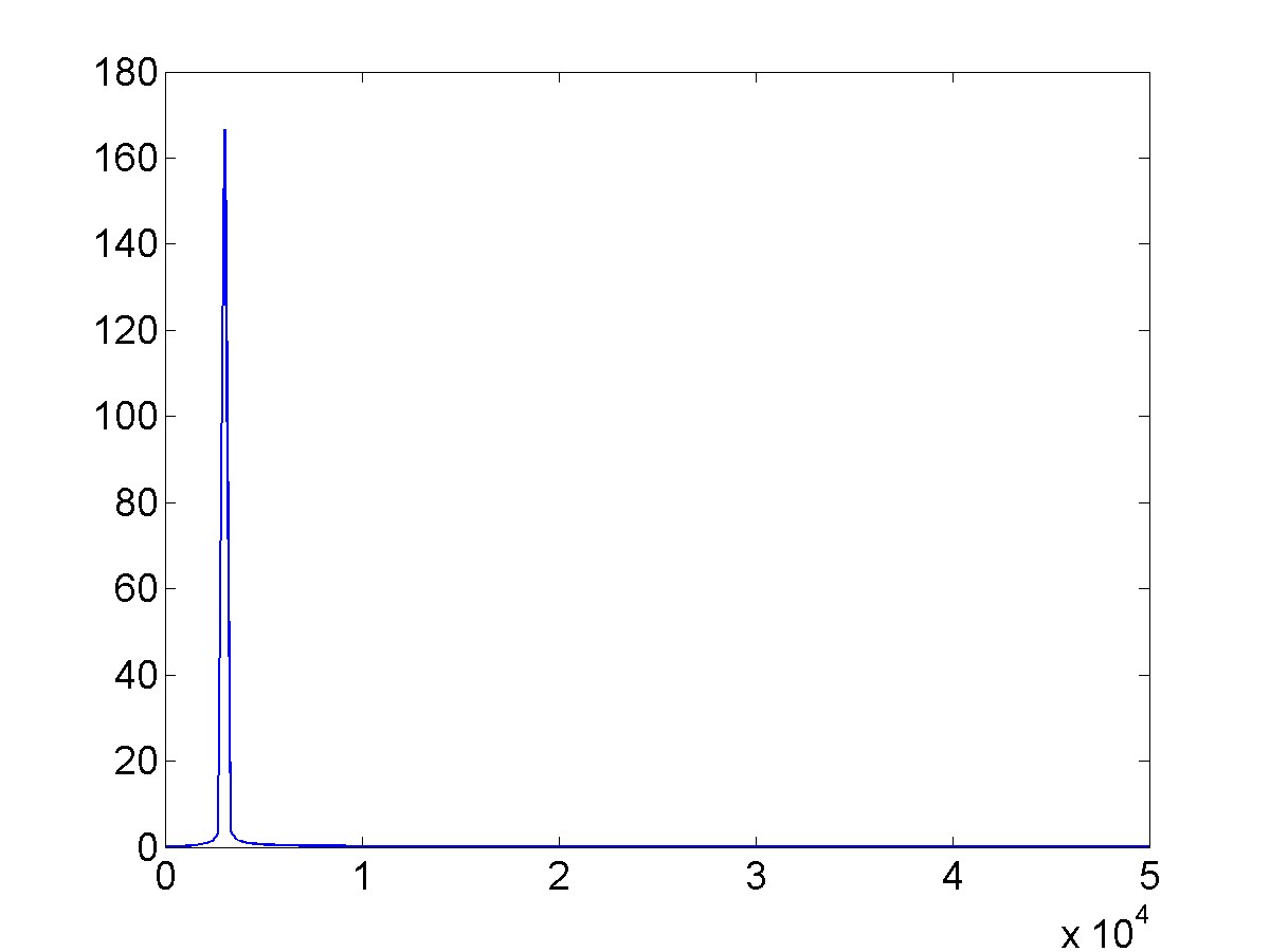
You can zoom in on the spike and verify that it has a frequency close to 3kHz.
Our signal does not have an amplitude greater than 100 so we obviously need to scale the amplitude. We simply need to divide the signal by the number of elements.
Y2 = Y1/(L/2);
plot(f,abs(Y2));
Here is the resulting plot.
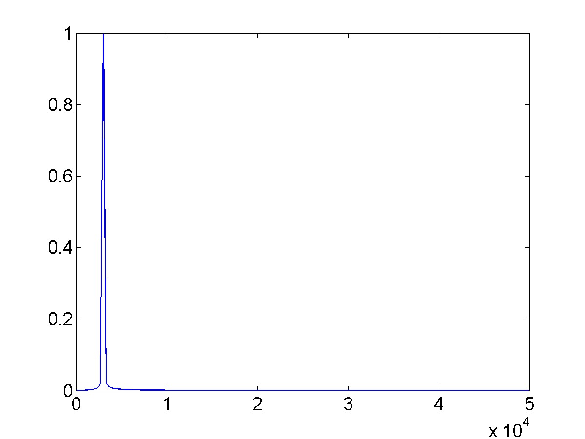
Zoom in on the spike to make sure that it is centered close to 3kHz.
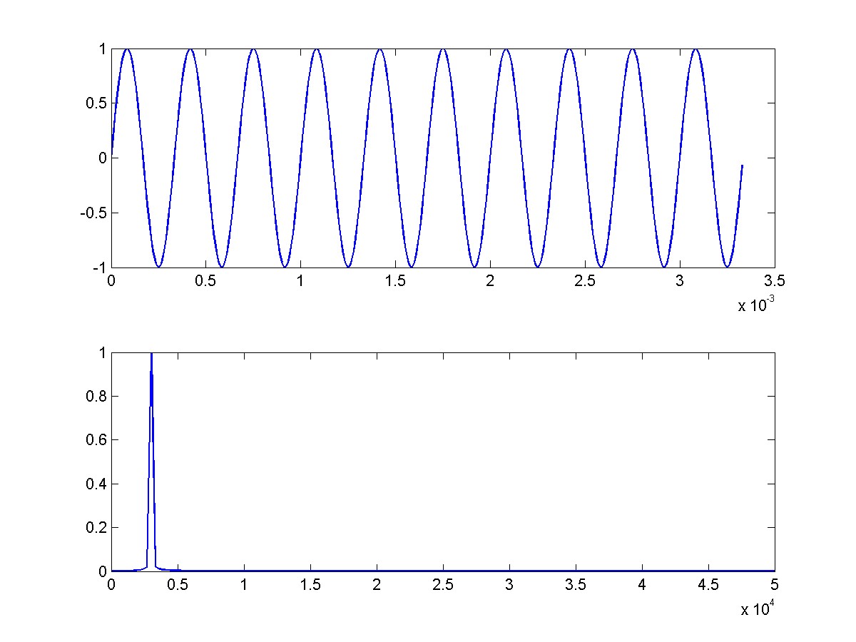
As you learned by watching the FFT video, the FFT creates an array of frequency domain spectrum samples. The number of samples is the same as the length of your data (N) and the frequency range is based on the sampling frequency fmax=Fs/2. This means that the frequency bin is Fs/(2*N).
In our example the number of samples is L/2=167 and the frequency band is Fs/2=50kHz. This means that our frequency resolution is 299.4 Hz. If we increase the number of points in our time domain signal without increasing the total time of the signal then we are actually changing the sampling frequency, which would increase our total frequency band but not change our frequency resolution. In order to change the resolution we need to increase the total time width of our signal without changing the sampling frequency.
This MATLAB code produces a sine wave with 10 periods and a corresponding frequency resolution of 299 Hz.
Fs = 100e3; % sample rate
f1 = 3e3;   % signal frequency
A1 = 1;     % signal amplitude, peak amplitude not peak-to-peak
t  = 0:1/Fs:10/f1;
y  = A1*sin(2*pi*f1*t);
Y  = fft(y);
L  = length(Y); % the total length of our fft
Y1 = Y(1:L/2);  % take the first half of the vector
Y2 = Y1/(L/2);
f  = linspace(0,Fs/2,L/2);
subplot(2,1,1);
plot(t,y);
subplot(2,1,2);
plot(f,abs(Y2));
Here are the resulting time domain and frequency domain plots.
This MATLAB code produces a sine wave with 100 periods and a corresponding frequency resolution of 29.9 Hz.
Fs = 100e3; % sample rate
f1 = 3e3;   % signal frequency
A1 = 1;     % signal amplitude, peak amplitude not peak-to-peak
t  = 0:1/Fs:100/f1;
y  = A1*sin(2*pi*f1*t);
Y  = fft(y);
L  = length(Y); % the total length of our fft
Y1 = Y(1:L/2);  % take the first half of the vector
Y2 = Y1/(L/2);
f  = linspace(0,Fs/2,L/2);
subplot(2,1,1);
plot(t,y);
subplot(2,1,2);
plot(f,abs(Y2));
Here are the resulting plots.

Using freqz
Here is an example to show how to use the freqz function.
(1) We need to create the filter.
Fs = 10e3;      % sample rate of 10kHz
Wn = [1e3 2e3]; % bandpass filter with 1kHz < f < 2kHz
Wn = Wn/(Fs/2); % divide by half of the sampling frequency

[B,A] = butter(4,Wn); % create the filter
(2) Set up the frequency vector.
F = 0:Fs/(1000):Fs/2; % create the array of frequencies
In this example we are creating an array of frequencies between 0 and the maximum frequency, which is half of the sampling frequency.
(3) Use the freqz function to create the complex frequency response.
H = freqz(B,A,F,Fs); % create the complex frequency response
(4) Plot the magnitude of the complex frequency response.
plot(F,abs(H));
Here is the resulting plot.
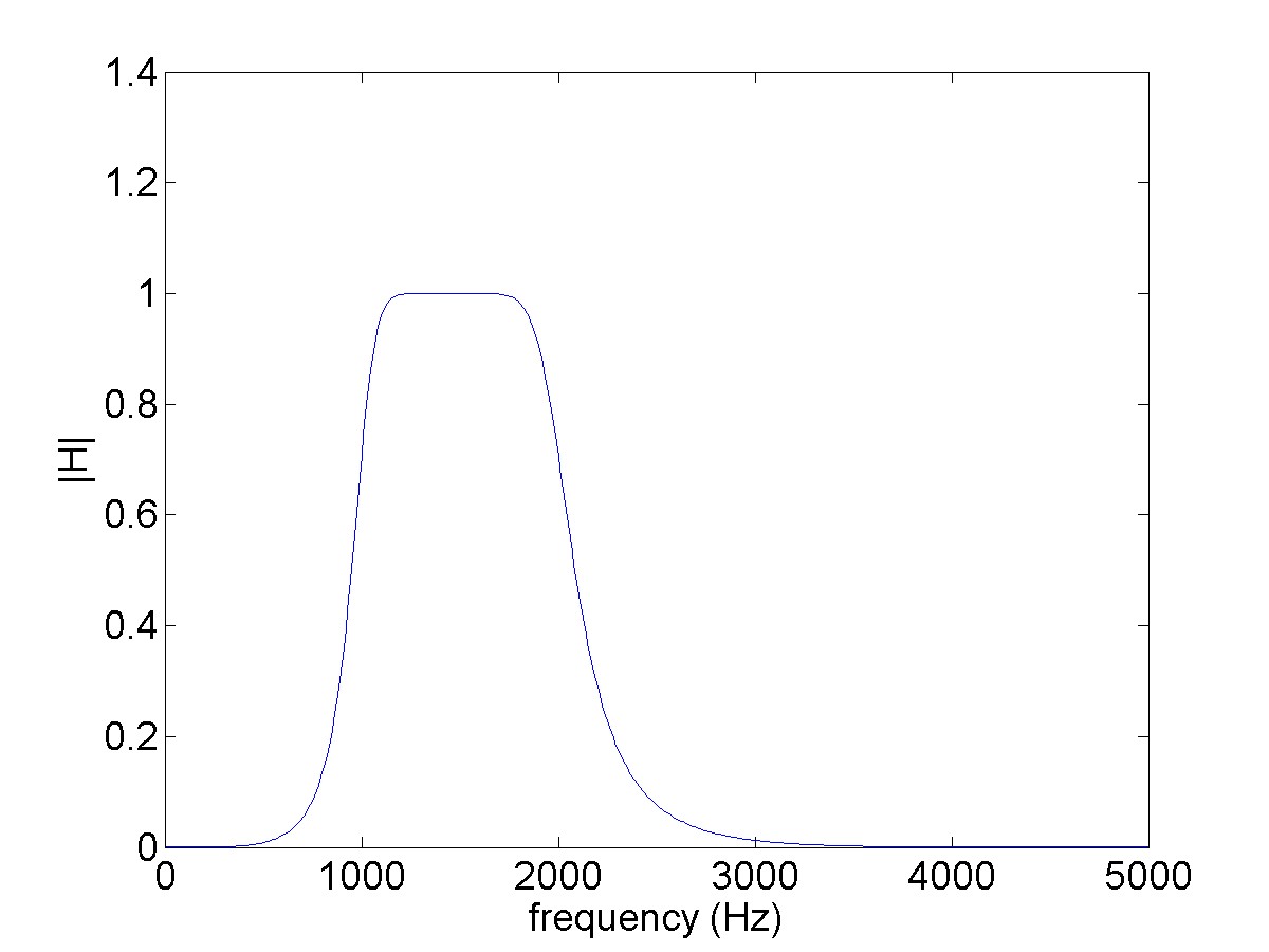
Notice how the filter is flat over the band between the two frequencies and then slopes down outside of this band. This is the shape of the frequency response of a bandpass filter.
Often the data is scaled to be in decibels so that it is easier to distinguish small changes. When you do this you often need to scale the y-axis of the plot to your desired range of interest.
H_db = 20*log10(abs(H));
plot(F,H_db);
axis([0 5000 -50 3]);
Here is the plot in decibel scale. You can zoom in on the 1kHz and 2kHz frequencies and see that these are the 3dB points.
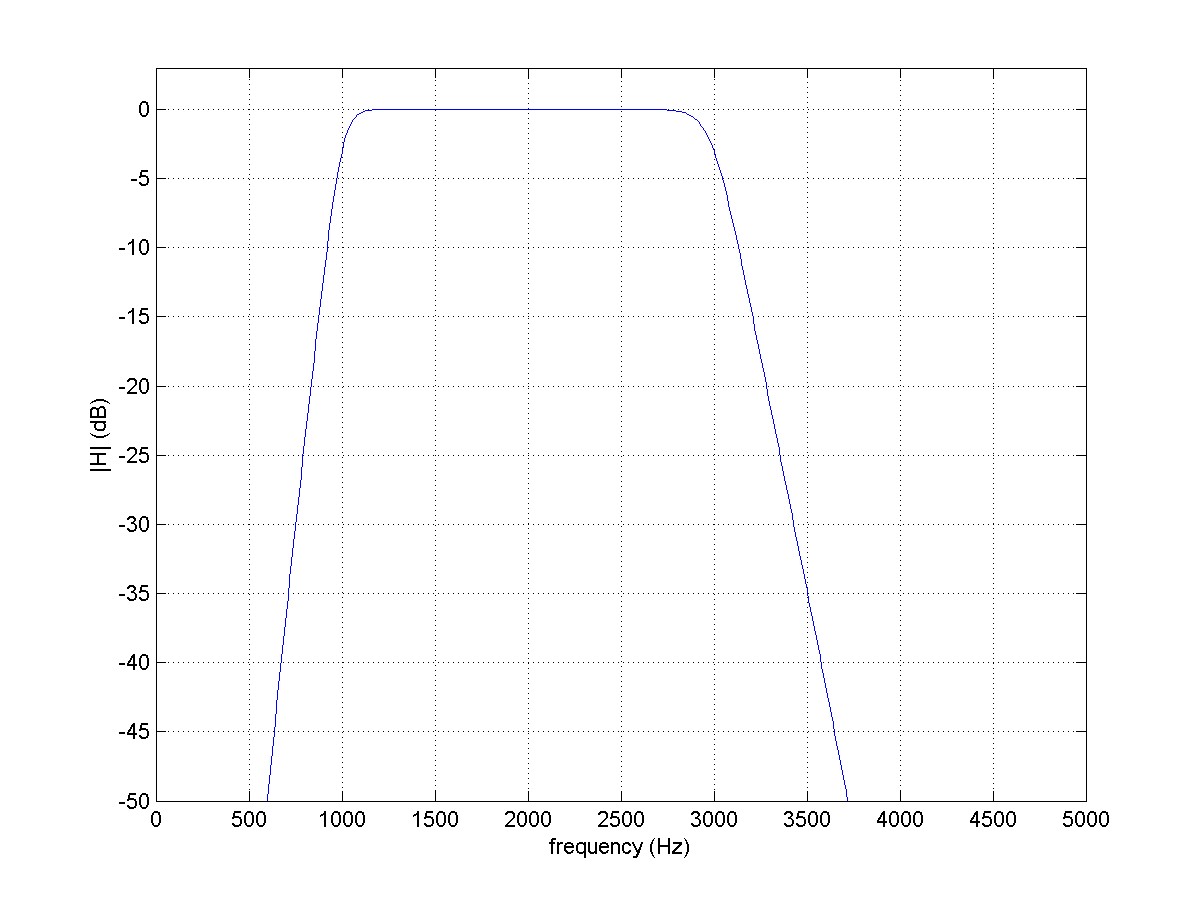
You can change the order of the filter and see that the filter becomes steeper and change the frequency corners and see the change in the width of the filter.