Table of Contents
In the previous tutorial, you learned about the three Tcl commands that you will use for simulation. In this tutorial, you will learn about additional features that hopefully will make it easier to write Tcl files.
Additional add_force Functionality
In the first tutorial, you saw this Tcl command:
add_force wireA 1
run 10ns

add_force wireA 0
run 10ns
While this is a simple approach, this could get really tedious if we were changing our signal often, or were working with a lot of signals. Fortunately there is a shorthand that saves a lot of typing:
add_force wireA {1 0ns} {0 10ns}

run 20ns
We still have the input name, wireA, but now we are writing out a signal and a timing in brackets {}. In this example, wireA will be set to 1 at 0ns and then set to 0 at 10ns. This pattern of {value timing} can be repeated as many times as needed. (Incidentally, the first assignment is assumed to start at time 0 if the timing isn’t stated, and the time is assumed to be measured in ns.)
# A condensed add_force command
add_force wireA {1} {0 10} {1 30} {0 35}

run 40
-repeat_every
While this is useful, sometimes we have signals that are changing constantly (usually this is your clock signal). The “-repeat_every” argument allows you to write an add_force command that repeats for as long as the simulation runs.
add_force clk {1} {0 5} -repeat_every 10
Here’s what this command is saying: set clk to 1 at 0ns, then to 0 at 5ns, and then at 10ns repeat this command. This means that clk will cycle from high to low every 10ns for as long as the simulation runs.
Additionally, it’s possible to use -repeat_every to simulate a truth table. This is useful if we want to exhaustively test a series of inputs.
restart

add_force A {0} {1 40} -repeat_every 80
add_force B {0} {1 20} -repeat_every 40
add_force C {0} {1 10} -repeat_every 20
add_force D {0} {1 5} -repeat_every 10

run 80
Here we have 4 input wires, each with a different add_force command. Notice that the -repeat_every lengths increase by a factor of 2 each time. Now look at this 4 input truth table:
| A | B | C | D |
|---|---|---|---|
| 0 | 0 | 0 | 0 |
| 0 | 0 | 0 | 1 |
| 0 | 0 | 1 | 0 |
| 0 | 0 | 1 | 1 |
| 0 | 1 | 0 | 0 |
| 0 | 1 | 0 | 1 |
| 0 | 1 | 1 | 0 |
| 0 | 1 | 1 | 1 |
| 1 | 0 | 0 | 0 |
| 1 | 0 | 0 | 1 |
| 1 | 0 | 1 | 0 |
| 1 | 0 | 1 | 1 |
| 1 | 1 | 0 | 0 |
| 1 | 1 | 0 | 1 |
| 1 | 1 | 1 | 0 |
| 1 | 1 | 1 | 1 |
Notice that A is 0 for the first half of the table and 1 for the second half, and that D switches every other row. Now look at this simulation:
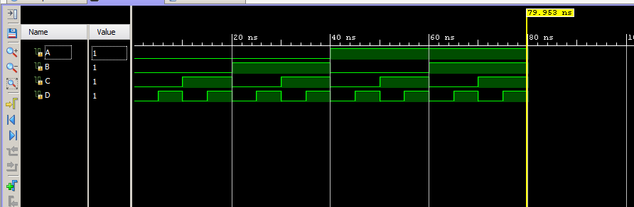
If you tilt your head, you can start to see the similarities between the waveform and the truth table.
Additional Tips
- Most of the modules you make will will have multi-bit inputs. These work exactly the same as single bit inputs and have the same syntax. Remember that add_force assumes binary values.
add_force sw 1000100010001111 add_force dataIn {0000} {1010 10} {1000 35} - That being said, it can be tedious to create add_force commands in binary for large wires. If you want to write values out in hex, use this syntax:
add_force -radix hex sw 888F add_force -radix hex dataIn {0} {A 10} {8 35} - Every time you change your code, you need to update your simulation. It can be quite frustrating if you forget to do this. Fortunately, there is a button at the top of the simulator that will relaunch and update your simulation. The other buttons there are also useful.

- When running a testbench, it often doesn’t run to completion. If you use the “run all” command, it will run until the testbench finishes. However, if the testbench gets stuck in an infinite loop (because your program has an unexpected error) it will never exit, so watch for that.